Create Space Time Cube From Defined Locations (Space Time Pattern Mining)—ArcGIS Pro

Summary

Takes panel data or station data (defined locations where geography does not change but attributes are changing over time) and structures it into a netCDF data format by creating space-time bins. For all locations, the trend for variables or summary fields is evaluated.

Learn more about how the Create Space Time Cube From Defined Locations works

Illustration

Usage

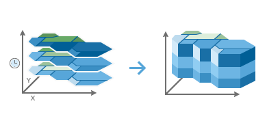
This tool takes panel or station data (defined locations where attributes are changing over time but geographies do not change) as Input Features and structures it into space-time bins. The data structure it creates can be thought of as a three-dimensional cube made up of space-time bins with the x and y dimensions representing space and the t dimension representing time.
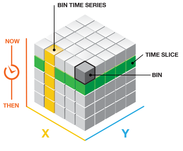
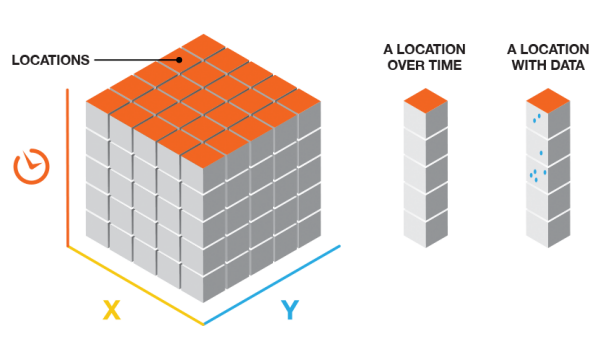
Every bin has a fixed position in space (x,y location if the inputs are points, and a fixed set of vertices if the inputs are polygon locations) and in time (t). Bins covering the same defined location area (either x,y or vertices) share the same Location ID. Bins encompassing the same duration share the same time-step ID.
Each bin in the space-time cube has a LOCATION_ID, time_step_ID, and COUNT value and values for any Variables or Summary Fields that were included when the cube was created. Bins associated with the same physical location will share the same location ID and together will represent a time series. Bins associated with the same time-step interval will share the same time-step ID and together will comprise a time slice.
The Input Features can be points or polygons and should represent defined or fixed locations with associated attributes that have been collected over time. This type of data is commonly called panel or station data. The field containing the event time stamp must be of type Date.
Note:
If your Input Features are stored in a file geodatabase and contain true curves (stored as arcs as opposed to stored with vertices), polygon shapes will be distorted when stored in the space-time cube. To check if your Input Features contain true curves, run the Check Geometry tool with the OGC Validation Method. If you receive an error message stating that the selected option does not support non-linear segments, then true curves exist in your dataset and may be eliminated and replaced with vertices by using the Densify tool with the Angle Densification Method before creating the space-time cube.
The Input Features can be repeating shapes contained within the same feature class or one set of features with a related table containing the attributes recorded over time.
The tool will fail if the parameters specified result in a cube with more than two billion bins.
This tool requires projected data to accurately measure distances.
If Temporal Aggregation is checked, the resulting space-time cube will contain a count value for each bin reflecting the number of events that occurred at the associated location within the associated time-step interval.
Output from this tool is a netCDF representation of your input features as well as messages summarizing cube characteristics. Messages are written at the bottom of the Geoprocessing pane during tool execution. You can access the messages by hovering over the progress bar, clicking the pop-out button , or expanding the messages section in the Geoprocessing pane. You can also access the messages for a previous run of the tool via the Geoprocessing History. You would use the netCDF file as input to other tools such as the Emerging Hot Spot Analysis tool or the Local Outlier Analysis tool. See Visualizing the Space Time Cube to get strategies allowing you to look at cube contents.
Select a field of type Date for the Time Field parameter. If the input is repeating shapes, this field should contain the timestamp associated with each feature. If the input has a Related Table, this field will be the timestamp associated with each record in the table.
The Time Step Interval defines how you want to partition the time span of your data. If Temporal Aggregation is checked off, the Time Step Interval should be set to the existing structure of your data. For instance, if you have census data that has been collected every five years, the input should be 5 years. Check on this parameter if you want to aggregate temporally. For instance, if you have sensor data that has been recording every 5 minutes, you might decide to aggregate using one-day intervals for example. Time-step intervals are always fixed durations, and the tool requires a minimum of ten time steps.
Note:
While a number of time units appear in the Time Step Interval drop-down list, the tool only supports Years, Months, Weeks, Days, Hours, Minutes, and Seconds.
If your space-time cube could not be created, the tool may have been unable to structure the input data you have provided into ten time-step intervals. If you receive an error message running this tool, examine the timestamps of the input to make sure they include a range of values (at least ten). The range of values must span at least 10 seconds as this is the smallest time increment that the tool will take. Ten time-step intervals are required by the Mann-Kendall statistic.
The Reference Time can be a date and time value or solely a date value; it cannot be solely a time value. The expected format is determined by the computer's regional time settings.
The trend analysis performed on the aggregated variables or summary field values is based on the Mann-Kendall statistic.
The following statistical operations are available for the aggregation of attributes with this tool: Sum, Mean, Minimum, Maximum, Standard Deviation, and Median.
Null values present in any of the summary field records will result in those features being excluded from the output cube. If there are null values present in your Input Features, it is highly recommended that you run the Fill Missing Values tool first. If, after running the Fill Missing Values tool, there are still null values present and having the count of points in each bin is part of your analysis strategy, you may want to consider creating separate cubes, one for the count (without Summary Fields) and one for Summary Fields. If the set of null values is different for each summary field, you may also consider creating a separate cube for each summary field.
When filling empty bins with SPATIAL_NEIGHBORS, the tool estimates based on the closest 8 nearest neighbors. A minimum of 4 of those spatial neighbors must have values to fill the empty bin using this option.
When filling empty bins with SPACE_TIME_NEIGHBORS, the tool estimates based on the closest 8 nearest neighbors. Additionally, temporal neighbors are used for each of those bins found to be spatial neighbors by going backward and forward 1 time step. A minimum of 13 space time neighbors are required to fill the empty bin using this option.
When filling empty bins with TEMPORAL_TREND, the first two time periods and last two time periods at a given location must have values in their bins to interpolate values at other time periods for that location.
The TEMPORAL_TREND fill type uses the Interpolated Univariate Spline method in the SciPy Interpolation package.
This tool can take advantage of the increased performance available in systems that use multiple CPUs (or multi-core CPUs). The tool will default to run using 50% of the processors available; however, the number of CPUs used can be increased or decreased using the Parallel Processing Factor environment. The increased processing speed is most noticeable when creating larger space-time cubes.

Syntax

CreateSpaceTimeCubeDefinedLocations(in_features, output_cube, location_id, temporal_aggregation, time_field, {time_step_interval}, {time_step_alignment}, {reference_time}, {variables}, {summary_fields}, {in_related_table}, {related_location_id})

Parameter	Explanation	Data Type
in_features	The input point or polygon feature class to be converted into a space-time cube.	Feature Layer
output_cube	The output netCDF data cube that will be created.	File
location_id	An integer field containing the ID number for each unique location.	Field
temporal_aggregation	APPLY_TEMPORAL_AGGREGATION —The space-time cube will temporally aggregate your features based on the time_step_interval you provide. For example, you have data that has been collected daily and want to create a cube with a weekly time_step_interval. NO_TEMPORAL_AGGREGATION —The space-time cube will be created using the existing temporal structure of your in_features. For example, you have yearly data and want to create a cube with a yearly time_step_interval. This is the default.	Boolean
time_field	The field containing the timestamp for each row in the dataset. This field must be of type Date.	Field
time_step_interval (Optional)	The number of seconds, minutes, hours, days, weeks, or years that will represent a single time step. Examples of valid entries for this parameter are 1 Weeks, 13 Days, or 1 Months. If temporal_aggregation is checked off, you are not aggregating temporally, and this parameter should be set to the existing temporal structure of your data. If temporal_aggregation is checked on, you are aggregating temporally, and this parameter should be set to the time_step_interval you want to create. All features within the same time_step_interval will be aggregated.	Time Unit
time_step_alignment (Optional)	Defines how the cube structure will occur based on a given time_step_interval. END_TIME —Time steps align to the last time event and aggregate back in time. START_TIME —Time steps align to the first time event and aggregate forward in time. REFERENCE_TIME —Time steps align to a particular date/time that you specify. If all points in the input features have a timestamp larger than the reference time you provide (or it falls exactly on the start time of the input features), the time-step interval will begin with that reference time and aggregate forward in time (as occurs with a START_TIME alignment). If all points in the input features have a timestamp smaller than the reference time you provide (or it falls exactly on the end time of the input features), the time-step interval will end with that reference time and aggregate backward in time (as occurs with an END_TIME alignment). If the reference time you provide is in the middle of the time extent of your data, a time-step interval will be created ending with the reference time provided (as occurs with an END_TIME alignment); additional intervals will be created both before and after the reference time until the full time extent of your data is covered.	String
reference_time (Optional)	The date/time to used to align the time-step intervals. If you want to bin your data weekly from Monday to Sunday, for example, you could set a reference time of Sunday at midnight to ensure bins break between Sunday and Monday at midnight.	Date
variables [[Field, Fill Empty Bins with],...] (Optional)	The numeric field containing attribute values that will be brought into the space-time cube. Available fill types are: DROP_LOCATIONS–Locations with missing data for any of the variables will be dropped from the output space-time cube. ZEROS–Fills empty bins with zeros. SPATIAL_NEIGHBORS–Fills empty bins with the average value of spatial neighbors. SPACE_TIME_NEIGHBORS–Fills empty bins with the average value of space time neighbors. TEMPORAL_TREND–Fills empty bins using an interpolated univariate spline algorithm. Note: Null values present in any of the variable records will result in an empty bin. If there are null values present in your input features, it is highly recommended that you run the Fill Missing Values tool first.	Value Table
summary_fields [[Field, Statistic, Fill Empty Bins with],...] (Optional)	The numeric field containing attribute values used to calculate the specified statistic when aggregating into a space-time cube. Multiple statistic and field combinations can be specified. Null values in any of the fields specified will result in that feature being dropped from the output cube. If there are null values present in your input features, it is highly recommended you run the Fill Missing Values tool before creating a space time cube. Available statistic types are: SUM–Adds the total value for the specified field within each bin. MEAN–Calculates the average for the specified field within each bin. MIN–Finds the smallest value for all records of the specified field within each bin. MAX–Finds the largest value for all records of the specified field within each bin. STD–Finds the standard deviation on values in the specified field within each bin. MEDIAN–Finds the sorted middle value of all records of the specified field within each bin. Available fill types are: ZEROS–Fills empty bins with zeros. SPATIAL_NEIGHBORS–Fills empty bins with the average value of spatial neighbors SPACE_TIME_NEIGHBORS–Fills empty bins with the average value of space time neighbors. TEMPORAL_TREND–Fills empty bins using an interpolated univariate spline algorithm. Note: Null values present in any of the summary field records will result in those features being excluded from the output cube. If there are null values present in your Input Features, it is highly recommended that you run the Fill Missing Values tool first. If, after running the Fill Missing Values tool, there are still null values present and having the count of points in each bin is part of your analysis strategy, you may want to consider creating separate cubes, one for the count (without Summary Fields) and one for Summary Fields. If the set of null values is different for each summary field, you may also consider creating a separate cube for each summary field.	Value Table
in_related_table (Optional)	The table or table view to be related to the input features.	Table View
related_location_id (Optional)	An integer field in the related table that contains the location ID on which the relate will be based.	Field

Code sample

CreateSpaceTimeCubeDefinedLocations example 1 (Python window)

The following Python window script demonstrates how to use the CreateSpaceTimeCubeDefinedLocations tool.

import arcpy
arcpy.env.workspace = r"C:\STPM\Chicago.gdb"
arcpy.CreateSpaceTimeCubeDefinedLocations_stpm("Chicago_Data", r"C:\STPM\Chicago_Cube.nc", "MYID",
                                               "NO_TEMPORAL_AGGREGATION", "TIME", "1 Months",
                                               "END_TIME", "", "COUNT ZEROS")

CreateSpaceTimeCubeDefinedLocations example 2 (stand-alone script)

The following stand-alone Python script demonstrates how to use the CreateSpaceTimeCubeDefinedLocations tool.

# Fill missing values using a feature set and related table
# Use the results to create a space-time cube from defined locations
# Run Emerging Hot Spot Analysis on the data
# Visualize the results in 3d

# Import system modules
import arcpy

# Set geoprocessor object property to overwrite existing output, by default
arcpy.env.overwriteOutput = True

# Local variables ...
arcpy.env.workspace = r"C:\STPM\Chicago.gdb"

try:

    # Fill missing values in a feature class containing block group polygon shapes and a related table containing the incidents
    # Since some of the values are missing we will fill them using the temporal trend method.

    arcpy.FillMissingValues_stpm("Chicago_Feature", "Chicago_FilledFeature", "COUNT", "TEMPORAL_TREND", "", "", NoneNone,
                                 "TIME", "", "MYID", "Chicago_Table", "MYID", "", "", "", "Chicago_FilledTable")



    # Create a defined location space time cube using a related table
    # Using a reference time at the start of the month to force binning fall on month breaks
    # Using temporal aggregation to sum multiple entries into one month
    # Using the method drop location if missing values since we already filled using Fill Missing Values
    arcpy.CreateSpaceTimeCubeDefinedLocations_stpm("Chicago_FilledFeature", r"C:\STPM\Chicago_Cube.nc", "MYID",
                                                   "APPLY_TEMPORAL_AGGREGATION", "TIME", "1 Months", "REFERENCE_TIME",
                                                   "10/1/2015", "", "COUNT SUM DROP_LOCATIONS", "Chicago_FilledTable",
                                                   "MYID")

    # Run an emerging hot spot analysis on the defined locations cube
    # Using contiguity edges so only block groups which bound each other are considered neighbours
    arcpy.EmergingHotSpotAnalysis_stpm(r"C:\STPM\Chicago_Cube.nc", "COUNT_SUM_NONE",
                                       "Chicago_Cube_EmergingHotSpot", "", 1, "",
                                       "CONTIGUITY_EDGES_ONLY")

    # Use Visualize Cube in 3d to see the hot spot results for each time slice
    arcpy.VisualizeSpaceTimeCube3D_stpm(r"C:\STPM\Chicago_Cube.nc", "COUNT_SUM_NONE", "HOT_AND_COLD_SPOT_RESULTS",
                                        "Chicago_Cube_Visualize3d")

except arcpy.ExecuteError:
    # If any error occurred when running the tool, print the messages
    print(arcpy.GetMessages())

Environments

Current Workspace, Scratch Workspace, Output Coordinate System, Geographic Transformations, Parallel Processing Factor

Licensing information

Basic: Yes
Standard: Yes
Advanced: Yes

Summary

Illustration

Usage

Note:

Note:

Syntax

Note:

Note:

Code sample

Environments

Licensing information

Related topics

In this topic