Summary
Finds spatially contiguous clusters of features based on a set of feature attribute values and optional cluster size limits.
Learn more about how Spatially Constrained Multivariate Clustering works
Illustration

Usage
-
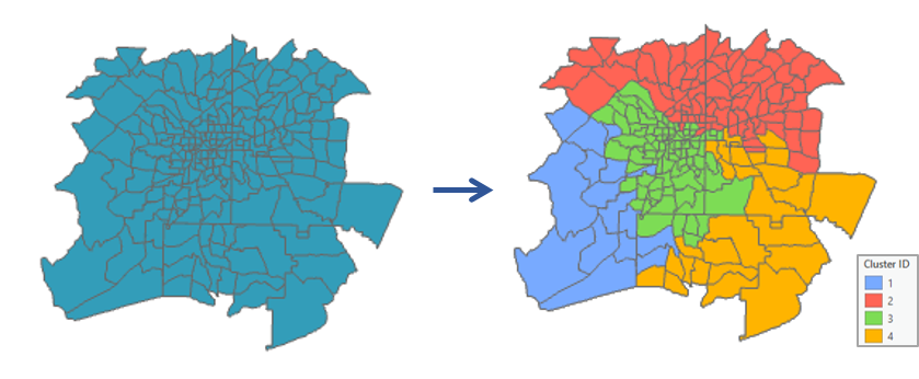
This tool produces an output feature class with the fields used in the analysis plus a new integer field named CLUSTER_ID. Default rendering is based on the CLUSTER_ID field and shows you which cluster each feature falls into. If you indicate that you want three clusters, for example, each record will contain a 1, 2, or 3 for the CLUSTER_ID field.
- Input can be points or polygons.
-
This tool also creates messages and charts to help you understand the characteristics of the clusters identified. You may access the messages by hovering over the progress bar, clicking on the pop-out button, or expanding the messages section in the Geoprocessing pane. You may also access the messages for a previous run of the Spatially Constrained Multivariate Clustering tool via the geoprocessing history. The charts created can be accessed from the Contents pane.
-
The Analysis Fields should be numeric and should contain a variety of values. Fields with no variation (that is, the same value for every record) will be dropped from the analysis but will be included in the Output Features. Categorical fields may be used with the tool if they are represented as dummy variables (a value of one for all features in a category and zeros for all other features).
-
The Spatially Constrained Multivariate Clustering tool will construct clusters with space (and potentially time constraints, when using a spatial weights matrix). For some applications, you may not want to impose contiguity or other proximity requirements on the clusters created. In those cases, use the Multivariate Clustering tool to create clusters with no spatial constraint.
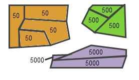
The size of the clusters can be managed with the Cluster Size Constraints parameter. You can set minimum and maximum thresholds that each cluster must meet. The size constraints can be either the Number of Features that each cluster contains or the sum of an Attribute Value. For example, if you cluster U.S. counties based on a set of economic variables, you can specify that each cluster has a minimum population of 5 million and a maximum population of 25 million.
When a Fill to Limit constraint is specified, the algorithm starts with a single cluster and will split clusters and solve until each of the clusters are below the Fill to Limit value, taking into account all of the variables with each split. The splitting will stop once the constraint is met, even if splitting existing clusters further may provide a better result.
If both a maximum and minimum are set to values close to each other, the Cluster Size Constraints parameter value for one of the resulting clusters may not be met.
Occasionally, the Cluster Size Constraints parameter may not be honored for all clusters due to the way the minimum spanning tree is constructed. The tool will finish, and the cluster that did not meet the size constraints will be reported in the messages.
-
This tool creates clusters that are spatially contiguous. The contiguity options enabled for polygon feature classes indicate features can be part of the same cluster only if they share an edge (Contiguity edges only) or if they share either an edge or a vertex (Contiguity edges corners) with another member of the cluster. The Trimmed Delaunay triangulation option ensures that outlier or island features can be clustered and may form disconnected clusters.
The default Spatial Constraints for point Input Features is Trimmed Delaunay triangulation, which will ensure all cluster members are proximal and that a feature will only be included in a cluster if at least one other feature is a natural neighbor. This method uses Delaunay triangulation to find point neighbors then crops the triangles with a convex hull. This ensures that point features cannot be neighbors with any features outside the convex hull.
The Trimmed Delaunay triangulation option ensures that neighboring features are in close proximity to each other. If there are spatial outliers in your data, this method may have little effect. This is because the Delaunay triangles extend so far out that the convex hull trimming has little effect on features that may not be in close proximity without the spatial outliers.
-
Additional Spatial Constraints, such as fixed distance or K nearest neighbors, can be imposed using the Generate Spatial Weights Matrix tool to first create a spatial weights matrix file (.swm) and then providing the path to that file for the Spatial Weights Matrix File parameter.
Note:
Even though you can create a spatial weights matrix (SWM) file to define spatial constraints, there is no actual weighting applied. The relationships become binary when defining spatial constraints within the clustering algorithm, even if a method such as Inverse Distance is used. If Inverse Distance is used without a distance cutoff, the result is a SWM that defines features based on weights, but the clustering algorithm ignores those weights and defines every feature as a neighbor of every other feature. This can impact performance and will lead to groups that are not truly spatially constrained. Similarly, choosing a K nearest neighbors conceptualization can result in clusters that are spatially constrained but not necessarily contiguous.
-
To create clusters with both space and time constraints, use the Generate Spatial Weights Matrix tool to first create a spatial weights matrix file (.swm) defining the space-time relationships among your features. Next, run the Spatially Constrained Multivariate Clustering tool, setting the Spatial Constraints parameter to Get spatial weights from file and the Spatial Weights Matrix File parameter to the SWM file you created.
To create three-dimensional clusters that take into consideration the z-values of your features, use the Generate Spatial Weights Matrix tool with the Use Z values parameter checked to first create a spatial weights matrix file (.swm), defining the 3D relationships among your features. Next, run Spatially Constrained Multivariate Clustering, setting the Spatial Constraints parameter to Get spatial weights from file and the Spatial Weights Matrix File parameter to the SWM file you created.
This tool is memory dependent. When using a Spatial Weights Matrix, a conceptualization of spatial relationships that results in each feature having a large number of neighbors will increase the likelihood of running into memory issues.
Defining a spatial constraint ensures compact, contiguous, or proximal clusters. Including spatial variables in your list of Analysis Fields can also encourage these cluster attributes. Examples of spatial variables are distance to freeway on-ramps, accessibility to job openings, proximity to shopping opportunities, measures of connectivity, and even coordinates (X, Y). Including variables representing time, day of the week, or temporal distance can encourage temporal compactness among cluster members.
-
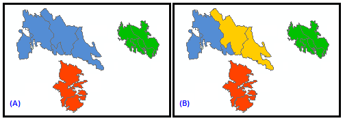
When there is a distinct spatial pattern to your features (three separate, spatially distinct clusters, for example), it can complicate the spatially constrained clustering algorithm. Consequently, the clustering algorithm first determines if there are any disconnected clusters. If the number of disconnected clusters is larger than the Number of Clusters specified, the tool cannot solve and will fail with an appropriate error message. If the number of disconnected clusters is the same as the Number of Clusters specified, the spatial configuration of the features alone determines cluster results, as shown in image (A) below. If the Number of Clusters specified is larger than the number of disconnected clusters, clustering begins with the disconnected clusters already determined. For example, if there are three disconnected clusters and the Number of Clusters specified is 4, one of the three clusters will be divided to create a fourth cluster, as shown in image (B) below.

-
In some cases, the Spatially Constrained Multivariate Clustering tool will not be able to meet the spatial constraints imposed, and features without neighbors will be the only feature in their cluster. Setting the Spatial Constraints parameter to Trimmed Delaunay triangulation can help resolve issues with disconnected clusters.
-
While there is a tendency to want to include as many Analysis Fields as possible, this tool works best when you start with a single variable and build. Results are easier to interpret with fewer analysis fields. It is also easier to determine which variables are the best discriminators when there are fewer fields.
-
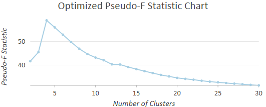
Sometimes you know the Number of Clusters most appropriate for your data. If you don't, however, you may have to try different numbers of clusters, noting which values provide the best group differentiation. When you leave the Number of Clusters parameter empty, the tool will evaluate the optimal number of clusters by computing a pseudo F-statistic for clustering solutions with 2 through 30 clusters and report the optimal number of clusters in the messages window. When you specify an optional Output Table for Evaluating Number of Clusters parameter value, a chart will be created showing the F-statistic values for solutions with 2 through 30 clusters. The largest F-statistic values indicate solutions that perform best at maximizing both within-cluster similarities and between-cluster differences. If no other criteria guide your choice for Number of Clusters, use a number associated with one of the largest pseudo F-statistic values.

-
Regardless of the Number of Clusters you specify, the tool will stop if division into additional clusters becomes arbitrary. For example, your data consists of three spatially clustered polygons and a single analysis field. If all the features in a cluster have the same analysis field value, it becomes arbitrary how any one of the individual clusters is divided after three groups have been created. If you specify more than three clusters in this situation, the tool will still only create three clusters. As long as at least one of the analysis fields in a cluster has some variation of values, division into additional clusters can continue.

Clusters will not be divided further if there is no variation in the analysis field values. -
When you include a spatial or space-time constraint in your analysis, the pseudo F-statistic values are comparable (as long as the Input Features and Analysis Fields don't change). Consequently, you can use the F-statistic values to determine not only optimal Number of Clusters but also to help you determine the most effective Spatial Constraints option.
-
The cluster number assigned to a set of features may change from one run to the next. For example, if you partition features into two clusters based on an income variable, the first time you run the analysis you might see the high income features labeled as cluster 2 and the low income features labeled as cluster 1. The second time you run the same analysis, the high income features might be labeled as cluster 1. You might also see that some of the middle income features switch cluster membership from one run to another.
The Permutations to Calculate Membership Probabilities parameter uses permutations and evidence accumulation to calculate the probability of cluster membership for each feature. A high probability tells you that you can be confident the feature belongs in the cluster it was assigned. A low probability may indicate the feature is very different than the cluster it was assigned or that the feature may be included in a different cluster if the Analysis Fields, Cluster Size Constraints, or Spatial Constraints parameter values were changed in some way. Calculating these probabilities uses permutations of random spanning trees and evidence accumulation. This can take significant time to run for larger datasets. It is recommended that you iterate and find the optimal number of clusters for your analysis first; then calculate probabilities for your analysis in a subsequent run. You can also increase performance by increasing the Parallel Processing Factor environment.
-
When the Input Features are not projected (that is, when coordinates are given in degrees, minutes, and seconds) or when the output coordinate system is set to a geographic coordinate system, distances are computed using chordal measurements. Chordal distance measurements are used because they can be computed quickly and provide very good estimates of true geodesic distances, at least for points within about 30 degrees of each other. Chordal distances are based on an oblate spheroid. Given any two points on the earth's surface, the chordal distance between them is the length of a line, passing through the three-dimensional earth, to connect those two points. Chordal distances are reported in meters.
Caution:
It is best practice to project your data, especially if your study area extends beyond 30 degrees. Chordal distances are not a good estimate of geodesic distances beyond 30 degrees.
This tool supports parallel processing to calculate probabilities and uses 50 percent of available processors by default. The number of processors can be increased or decreased using the Parallel Processing Factor environment.
Syntax
SpatiallyConstrainedMultivariateClustering(in_features, output_features, analysis_fields, {size_constraints}, {constraint_field}, {min_constraint}, {max_constraint}, {number_of_clusters}, {spatial_constraints}, {weights_matrix_file}, {number_of_permutations}, output_table)| Parameter | Explanation | Data Type |
in_features | The feature class or feature layer for which you want to create clusters. | Feature Layer |
output_features | The new output feature class created containing all features, the analysis fields specified, and a field indicating to which cluster each feature belongs. | Feature Class |
analysis_fields [analysis_fields,...] | A list of fields that will be used to distinguish one cluster from another. | Field |
size_constraints (Optional) | Specifies cluster size based on number of features per group or a target attribute value per group.
| String |
constraint_field (Optional) | The attribute value to be summed per cluster. | Field |
min_constraint (Optional) | The minimum number of features per cluster or the minimum attribute value per cluster. This must be a positive value. | Double |
max_constraint (Optional) | The maximum number of features per cluster or the maximum attribute value per cluster. If a maximum constraint is set, the number_of_clusters parameter is disabled. This must be a positive value. | Double |
number_of_clusters (Optional) | The number of clusters to create. If this parameter is empty, the tool will evaluate the optimal number of clusters by computing a pseudo F-statistic value for clustering solutions with 2 through 30 clusters. This parameter will be disabled if a maximum number of features or maximum attribute value has been set. | Long |
spatial_constraints (Optional) | Specifies how spatial relationships among features will be defined.
| String |
weights_matrix_file (Optional) | The path to a file containing spatial weights that define spatial, and potentially temporal, relationships among features. | File |
number_of_permutations (Optional) | The number of random permutations for the calculation of membership stability scores. If 0 (zero) is chosen, probabilities will not be calculated. Calculating these probabilities uses permutations of random spanning trees and evidence accumulation. This calculation can take a significant time to run for larger datasets. It is recommended that you iterate and find the optimal number of clusters for your analysis first; then calculate probabilities for your analysis in a subsequent run. Setting the Parallel Processing Factor Environment setting to 50 may improve the run time of the tool. | Long |
output_table | The table created containing the results of the F-statistic values calculated to evaluate the optimal number of clusters. The chart created from this table can be accessed in the Contents pane under the output feature layer. | Table |
Code sample
The following Python window script demonstrates how to use the SpatiallyConstrainedMultivariateClustering tool.
import arcpy
arcpy.env.workspace = r"C:\Analysis
arcpy.SpatiallyConstrainedMultivariateClustering_stats("CA_schools", "CA_Schools_100k_Students", "NumStudent",
                                          "ATTRIBUTE_VALUE", "NumStudent", 100000, None, None,
"CONTIGUITY_EDGES_CORNERS")The following Python script demonstrates how to use the SpatiallyConstrainedMultivariateClustering tool.
# Creating regions of similar schools districts with at least 100,0000 students each
# Import system modules
import arcpy

# Set property to overwrite existing output, by default
arcpy.env.overwriteOutput = True

# Local variables...
workspace = r"E:\working\data.gdb"
arcpy.env.workspace = workspace

# Create clusters of schools with a minimum of 100,000 students
arcpy.stats.SpatiallyConstrainedMultivariateClustering("CA_schools", "CA_Schools_100k_Students", "NumStudent",
                                          "ATTRIBUTE_VALUE", "NumStudent", 100000, None, None,
                                          "CONTIGUITY_EDGES_CORNERS")

# Create a spatial weights matrix using k nearest neighbors 16 to have more control over the search neighborhood
arcpy.stats.GenerateSpatialWeightsMatrix(r"E:\working\data.gdb\CA_schools", "UID",
                                         r"E:\working\schools_knn_16.swm", "K_NEAREST_NEIGHBORS", "EUCLIDEAN", 1,
                                         None, 16, "NO_STANDARDIZATION", None, None, None, None, "DO_NOT_USE_Z_VALUES")

# Create clusters again this time using the SWM file for search neighborhood and a maximum number
# of students per cluster
arcpy.stats.SpatiallyConstrainedMultivariateClustering("CA_schools", "CA_Schools_SWM_Knn16", "NumStudent", "ATTRIBUTE_VALUE",
                                          "NumStudent", None, 250000, None, "GET_SPATIAL_WEIGHTS_FROM_FILE",
                                          r"E:\working\schools_knn_16.swm")

# Use Summary Statistics with Cluster ID as a case field to see how many students were assigned to each cluster
arcpy.analysis.Statistics("CA_Schools_SWM_Knn16", "School_SummaryStatistics", "NumStudent SUM", "CLUSTER_ID")
Environments
- Output Coordinate System
Feature geometry is projected to the Output Coordinate System prior to analysis. All mathematical computations are based on the Output Coordinate System spatial reference. When the Output Coordinate System is based on degrees, minutes, and seconds, geodesic distances are estimated using chordal distances.
- Random number generator
The Random Generator Type used is always Mersenne Twister.
Licensing information
- Basic: Yes
- Standard: Yes
- Advanced: Yes