Warp From File (Data Management)

Summary

Transforms a raster dataset using an existing text file containing source and target control points.

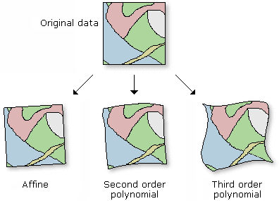
Illustration

Usage

• Warp is useful when the raster requires a systematic geometric correction that can be modeled with a polynomial. A spatial transformation can invert or remove a distortion using polynomial transformation of the proper order. The higher the order, the more complex the distortion that can be corrected. The higher orders of polynomial will involve progressively more processing time.

• The default polynomial order will perform an affine transformation.

• To determine the minimum number of links necessary for a given order of polynomial, use the following formula:

  n = (p + 1) (p + 2) / 2

  where n is the minimum number of links required for a transformation of polynomial order p. It is suggested that you use more than the minimum number of links.

• This tool will determine the extent of the warped raster and will set the number of rows and columns to be about the same as in the input raster. Some minor differences may be due to the changed proportion between the output raster's sizes in the x and y directions. The default cell size used will be computed by dividing the extent by the previously determined number of rows and columns. The value of the cell size will be used by the resampling algorithm.

  If you choose to define an output cell size in the Environment settings, the number of rows and columns will be calculated as follows:

• You can save your output to BIL, BIP, BMP, BSQ, DAT, Esri Grid , GIF, IMG, JPEG, JPEG 2000, PNG, TIFF, MRF, CRF, or any geodatabase raster dataset.

• When storing your raster dataset to a JPEG file, a JPEG 2000 file, or a geodatabase, you can specify a Compression Type and Compression Quality in the Environments.

• Each row in the input link file should have the following values, each delimited by a TAB:

  <From X> <From Y> <To X> <To Y>

  where each row represents the coordinates of a control point pair. There can be additional columns with residual values, but these are not required.

• This tool supports multidimensional raster data. To run the tool on each slice in the multidimensional raster and generate a multidimensional raster output, be sure to save the output to CRF.

  Supported input multidimensional dataset types include multidimensional raster layer, mosaic dataset, image service, and CRF.

Parameters

Dialog

Label	Explanation	Data Type
Input Raster	The raster to be transformed.	Mosaic Layer; Raster Layer
Output Raster Dataset	The name, location, and format for the dataset you are creating. When storing a raster dataset in a geodatabase, do not add a file extension to the name of the raster dataset. When storing your raster dataset to a JPEG file, a JPEG 2000 file, a TIFF file, or a geodatabase, you can specify a compression type and compression quality using environment settings. .bil—Esri BIL .bip—Esri BIP .bmp—BMP .bsq—Esri BSQ .dat—ENVI DAT .gif—GIF .img—ERDAS IMAGINE .jpg—JPEG .jp2—JPEG 2000 .png—PNG .tif—TIFF .mrf—MRF .crf—CRF No extension for Esri Grid	Raster Dataset
Link File	The text, CSV file, or TAB file containing the coordinates to warp the input raster. This can be generated from the Register Raster tool or from the Georeferencing tab.	Text File
Transformation Type (Optional)	Specifies the transformation method for shifting the raster dataset. Shift only — This method uses a zero-order polynomial to shift your data. This is commonly used when your data is already georeferenced, but a small shift will better line up your data. Only one link is required to perform a zero-order polynomial shift. Affine transformation —A first-order polynomial (affine) fits a flat plane to the input points. Second-order polynomial transformation —A second-order polynomial fits a somewhat more complicated surface to the input points. Third-order polynomial transformation —A third-order polynomial fits a more complicated surface to the input points. Optimize for global and local accuracy — This method combines a polynomial transformation and uses a triangulated irregular network (TIN) interpolation technique to optimize for both global and local accuracy. Spline transformation — This method transforms the source control points precisely to the target control points. In the output, the control points will be accurate, but the raster pixels between the control points are not. Projective transformation — This method warps lines so they remain straight. In doing so, lines that were once parallel may no longer remain parallel. The projective transformation is especially useful for oblique imagery, scanned maps, and for some imagery products. Similarity transformation — This is a first order transformation that attempts to preserve the shape of the original raster. The RMS error tends to be higher than other polynomial transformations because the preservation of shape is more important than the best fit.	String
Resampling Technique (Optional)	The resampling algorithm to be used. The Nearest and Majority options are used for categorical data, such as a land-use classification. The Nearest option is the default since it is the quickest and also because it will not change the cell values. Do not use either of these for continuous data, such as elevation surfaces. The Bilinear option and the Cubic option are most appropriate for continuous data. It is recommended that neither of these be used with categorical data because the cell values may be altered. Nearest neighbor — Nearest neighbor is the fastest resampling method; it minimizes changes to pixel values since no new values are created. It is suitable for discrete data, such as land cover. Bilinear interpolation — Bilinear interpolation calculates the value of each pixel by averaging (weighted for distance) the values of the surrounding four pixels. It is suitable for continuous data. Cubic convolution — Cubic convolution calculates the value of each pixel by fitting a smooth curve based on the surrounding 16 pixels. This produces the smoothest image but can create values outside of the range found in the source data. It is suitable for continuous data. Majority resampling —Majority resampling determines the value of each pixel based on the most popular value in a 3 by 3 window. Suitable for discrete data.	String

Python

arcpy.management.WarpFromFile(in_raster, out_raster, link_file, {transformation_type}, {resampling_type})

Name	Explanation	Data Type
in_raster	The raster to be transformed.	Mosaic Layer; Raster Layer
out_raster	The name, location, and format for the dataset you are creating. When storing a raster dataset in a geodatabase, do not add a file extension to the name of the raster dataset. When storing your raster dataset to a JPEG file, a JPEG 2000 file, a TIFF file, or a geodatabase, you can specify a compression type and compression quality using environment settings. .bil—Esri BIL .bip—Esri BIP .bmp—BMP .bsq—Esri BSQ .dat—ENVI DAT .gif—GIF .img—ERDAS IMAGINE .jpg—JPEG .jp2—JPEG 2000 .png—PNG .tif—TIFF .mrf—MRF .crf—CRF No extension for Esri Grid	Raster Dataset
link_file	The text, CSV file, or TAB file containing the coordinates to warp the input raster. This can be generated from the Register Raster tool or from the Georeferencing tab.	Text File
transformation_type (Optional)	Specifies the transformation method for shifting the raster dataset. POLYORDER0 — This method uses a zero-order polynomial to shift your data. This is commonly used when your data is already georeferenced, but a small shift will better line up your data. Only one link is required to perform a zero-order polynomial shift. POLYSIMILARITY — This is a first order transformation that attempts to preserve the shape of the original raster. The RMS error tends to be higher than other polynomial transformations because the preservation of shape is more important than the best fit. POLYORDER1 —A first-order polynomial (affine) fits a flat plane to the input points. POLYORDER2 —A second-order polynomial fits a somewhat more complicated surface to the input points. POLYORDER3 —A third-order polynomial fits a more complicated surface to the input points. ADJUST — This method combines a polynomial transformation and uses a triangulated irregular network (TIN) interpolation technique to optimize for both global and local accuracy. SPLINE — This method transforms the source control points precisely to the target control points. In the output, the control points will be accurate, but the raster pixels between the control points are not. PROJECTIVE — This method warps lines so they remain straight. In doing so, lines that were once parallel may no longer remain parallel. The projective transformation is especially useful for oblique imagery, scanned maps, and for some imagery products.	String
resampling_type (Optional)	The resampling algorithm to be used. NEAREST — Nearest neighbor is the fastest resampling method; it minimizes changes to pixel values since no new values are created. It is suitable for discrete data, such as land cover. BILINEAR — Bilinear interpolation calculates the value of each pixel by averaging (weighted for distance) the values of the surrounding four pixels. It is suitable for continuous data. CUBIC — Cubic convolution calculates the value of each pixel by fitting a smooth curve based on the surrounding 16 pixels. This produces the smoothest image but can create values outside of the range found in the source data. It is suitable for continuous data. MAJORITY —Majority resampling determines the value of each pixel based on the most popular value in a 3 by 3 window. Suitable for discrete data. The Nearest and Majority options are used for categorical data, such as a land-use classification. The Nearest option is the default since it is the quickest and also because it will not change the cell values. Do not use either of these for continuous data, such as elevation surfaces. The Bilinear option and the Cubic option are most appropriate for continuous data. It is recommended that neither of these be used with categorical data because the cell values may be altered.	String

Code sample

WarpFromFile example 1 (Python window)

This is a Python sample for the WarpFromFile tool.

import arcpy
arcpy.WarpFromFile_management(
     "\\cpu\data\raster.img", "\\cpu\data\warp_out.tif",
     "\\cpu\data\gcpfile.txt", "POLYORDER2", "BILINEAR")

WarpFromFile example 2 (stand-alone script)

This is a Python script sample for the WarpFromFile tool.

##Warp image with signiture file

import arcpy
arcpy.env.workspace = r"C:/Workspace"
    
    
arcpy.WarpFromFile_management("raster.img", "warp_output.tif", "gcpfile.txt", 
                      "POLYORDER2", "BILINEAR")

Environments

Compression, Current Workspace, Extent, Geographic Transformations, NoData, Output CONFIG Keyword, Output Coordinate System, Parallel Processing Factor, Pyramid, Raster Statistics, Resampling Method, Scratch Workspace, Snap Raster, Tile Size

Licensing information

• Basic: Yes
• Standard: Yes
• Advanced: Yes