Generalized Linear Regression (GLR) (Spatial Statistics)—ArcGIS Pro

Summary

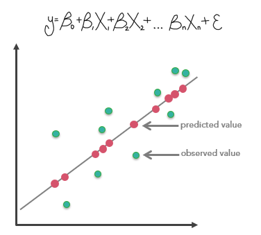
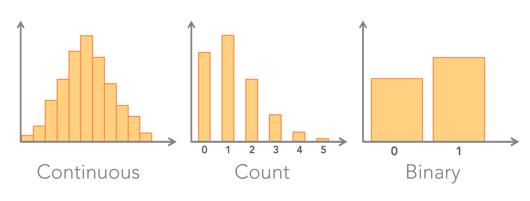
Performs Generalized Linear Regression (GLR) to generate predictions or to model a dependent variable in terms of its relationship to a set of explanatory variables. This tool can be used to fit continuous (OLS), binary (logistic), and count (Poisson) models.

Learn more about how Generalized Linear Regression works

Illustration

Usage

The primary output for this tool is a report file that is available as messages at the bottom of the Geoprocessing pane during tool execution. To access the messages, hove over the progress bar, click the pop-out button, or expand the messages section in the Geoprocessing pane. You can also access the messages of a previous run of the tool via the geoprocessing history.
Use the Input Features parameter with a field representing the phenomena you are modeling (the Dependent Variable) and one or more fields representing the Explanatory Variable(s). These fields must be numeric and have a range of values. Features that contain missing values in the dependent or explanatory variable will be excluded from the analysis; however, you can use the Fill Missing Values tool to complete the dataset before running the tool.
The Generalized Linear Regression tool also produces Output Features with coefficient information and diagnostics. The output feature class is automatically added to the table of contents with a rendering scheme applied to model residuals. A full explanation of each output is provided in How Generalized Linear Regression works.
The option you choose for the Model Type parameter depends on the data you are modeling. It is important to use the correct model for your analysis to obtain accurate results from your regression analysis.
Model summary results and diagnostics are written to the messages window and charts will be created below the output feature class. The diagnostics and charts reported depend on the Model Type parameter and are explained in detail in the How Generalized Linear Regression works topic.
Results from GLR are only trustworthy if your data and regression model satisfy all of the assumptions inherently required by this method. Be sure to check all resulting diagnostics and consult the Common regression problems, consequences, and solutions table in Regression analysis basics to ensure your model is properly specified.
The Dependent Variable and Explanatory Variable(s) parameters should be numeric fields containing a variety of values. This tool cannot solve when variables have the same values (all the values for a field are 9.0, for example).
Explanatory variables can come from fields or be calculated from distance features using the Explanatory Distance Features parameter. You can use a combination of these explanatory variable types, but at least one type is required. Explanatory Distance Features are used to automatically create explanatory variables representing a distance from the provided features to the Input Features. Distances will be calculated from each of the input Explanatory Distance Features to the nearest Input Features. If the input Explanatory Distance Features are polygons or lines, the distance attributes are calculated as the distance between the closest segments of the pair of features. However, distances are calculated differently for polygons and lines. See How proximity tools calculate distance for details.
It is recommended that you use projected data when Explanatory Distance Features are a component of the analysis. It is strongly recommended that your data be projected using a projected coordinate system (rather than a geographic coordinate system) to accurately measure distances.
When there is statistically significant spatial autocorrelation of the regression residuals, the GLR model will be considered incorrectly specified and, consequently, results from GLR are unreliable. Be sure to run the Spatial Autocorrelation tool on your regression residuals to assess this potential problem. Statistically significant spatial autocorrelation of regression residuals may indicate that one or more key explanatory variables are missing from the model.
You should visually inspect the over- and under-predictions evident in your regression residuals to see if they provide clues about potential missing variables from your regression model. It may help to run Hot Spot Analysis on the residuals to help you visualize spatial clustering of the over- and underpredictions.
When misspecification is the result of trying to model nonstationarity variables using a global model (GLR is a global model), the Geographically Weighted Regression tool can be used to improve predictions and to better understand the nonstationarity (regional variation) inherent in your explanatory variables.
When the result of a computation is infinity or undefined, the output for nonshapefiles will be Null; for shapefiles, the output will be -DBL_MAX (-1.7976931348623158e+308, for example).

Caution:

When using shapefiles, keep in mind that they cannot store null values. Tools or other procedures that create shapefiles from nonshapefile inputs may store or interpret null values as zero. In some cases, nulls are stored as very large negative values in shapefiles. This can lead to unexpected results. See Geoprocessing considerations for shapefile output for more information.

Parameters

Label	Explanation	Data Type
Input Features	The feature class containing the dependent and independent variables.	Feature Layer
Dependent Variable	The numeric field containing the observed values to be modeled.	Field
Model Type	Specifies the type of data that will be modeled. Continuous (Gaussian) — The dependent_variable is continuous. The model used is Gaussian, and the tool performs ordinary least squares regression. Binary (Logistic) — The dependent_variable represents presence or absence. This can be either conventional 1s and 0s, or continuous data that has been recoded based on some threshold value. The model used is Logistic Regression. Count (Poisson) —The dependent_variable is discrete and represents events, for example, crime counts, disease incidents, or traffic accidents. The model used is Poisson regression. Continuous (Gaussian) — The Dependent Variable is continuous. The model used is Gaussian, and the tool performs ordinary least squares regression. Binary (Logistic) — The Dependent Variable represents presence or absence. This can be either conventional 1s and 0s, or continuous data that has been recoded based on some threshold value. The model used is Logistic Regression. Count (Poisson) —The Dependent Variable is discrete and represents events, for example, crime counts, disease incidents, or traffic accidents. The model used is Poisson regression.	String
Output Features	The new feature class that will contain the dependent variable estimates and residuals.	Feature Class
Explanatory Variable(s)	A list of fields representing independent explanatory variables in the regression model.	Field
Explanatory Distance Features (Optional)	Automatically creates explanatory variables by calculating a distance from the provided features to the Input Features. Distances will be calculated from each of the input Explanatory Distance Features to the nearest Input Features. If the input Explanatory Distance Features are polygons or lines, the distance attributes are calculated as the distance between the closest segments of the pair of features.	Feature Layer
Prediction Locations (Optional)	A feature class containing features representing locations where estimates will be computed. Each feature in this dataset should contain values for all the explanatory variables specified. The dependent variable for these features will be estimated using the model calibrated for the input feature class data.	Feature Layer
Match Explanatory Variables (Optional)	Matches the explanatory variables in the Prediction Locations to corresponding explanatory variables from the Input Feature Class.	Value Table
Match Distance Features (Optional)	Matches the distance features specified for the Prediction Locations on the left to corresponding distance features for the Input Features on the right.	Value Table
Output Predicted Features (Optional)	The output feature class to receive dependent variable estimates for each Prediction Location.	Feature Class

arcpy.stats.GeneralizedLinearRegression(in_features, dependent_variable, model_type, output_features, explanatory_variables, {distance_features}, {prediction_locations}, {explanatory_variables_to_match}, {explanatory_distance_matching}, {output_predicted_features})

Name	Explanation	Data Type
in_features	The feature class containing the dependent and independent variables.	Feature Layer
dependent_variable	The numeric field containing the observed values to be modeled.	Field
model_type	Specifies the type of data that will be modeled. CONTINUOUS — The dependent_variable is continuous. The model used is Gaussian, and the tool performs ordinary least squares regression. BINARY — The dependent_variable represents presence or absence. This can be either conventional 1s and 0s, or continuous data that has been recoded based on some threshold value. The model used is Logistic Regression. COUNT —The dependent_variable is discrete and represents events, for example, crime counts, disease incidents, or traffic accidents. The model used is Poisson regression.	String
output_features	The new feature class that will contain the dependent variable estimates and residuals.	Feature Class
explanatory_variables [explanatory_variables,...]	A list of fields representing independent explanatory variables in the regression model.	Field
distance_features [distance_features,...] (Optional)	Automatically creates explanatory variables by calculating a distance from the provided features to the in_features. Distances will be calculated from each of the input distance_features to the nearest in_features. If the input distance_features are polygons or lines, the distance attributes are calculated as the distance between the closest segments of the pair of features.	Feature Layer
prediction_locations (Optional)	A feature class containing features representing locations where estimates will be computed. Each feature in this dataset should contain values for all the explanatory variables specified. The dependent variable for these features will be estimated using the model calibrated for the input feature class data.	Feature Layer
explanatory_variables_to_match [[Field from Prediction Locations, Field from Input Features],...] (Optional)	Matches the explanatory variables in the prediction_locations to corresponding explanatory variables from the in_features—for example, [["LandCover2000", "LandCover2010"], ["Income", "PerCapitaIncome"]]	Value Table
explanatory_distance_matching [[Prediction Distance Features, Input Explanatory Distance Features],...] (Optional)	Matches the distance features specified for the features_to_predict on the left to the corresponding distance features for the in_features on the right—for example, [["stores2010", "stores2000"], ["freeways2010", "freeways2000"]].	Value Table
output_predicted_features (Optional)	The output feature class to receive dependent variable estimates for each prediction_location. The output feature class to receive dependent variable estimates for each Prediction Location.	Feature Class

Code sample

GeneralizedLinearRegression example 1 (Python window)

The following Python window script demonstrates how to use the GeneralizedLinearRegression tool.

import arcpy
arcpy.env.workspace = r"c:\data\project_data.gdb"
arcpy.stats.GeneralizedLinearRegression("landslides", "occurred",
                                 "BINARY", "out_features", 
                                 "eastness;northness;elevation;slope", 
                                 "rivers")

GeneralizedLinearRegression example 2 (stand-alone script)

The following stand-alone Python script demonstrates how to use the GeneralizedLinearRegression tool.

# Linear regression using a count model to predict the number of crimes.
# The depend variable (total number of crimes) is predicted using total
# population, the median age of housing, average household income and the
# distance to the central business district (CBD)

import arcpy

# Set the current workspace (to avoid having to specify the full path to
# the feature classes each time)
arcpy.env.workspace = r"c:\data\project_data.gdb"

arcpy.stats.GeneralizedLinearRegression("crime_counts", 
     "total_crimes", "COUNT", "out_features", "YRBLT;TOTPOP;AVGHINC", 
     "CBD", "prediction_locations", "YRBLT YRBLT;TOTPOP TOTPOP;AVGHINC AVGHINC", 
     "CBD CBD", "predicted_features")

Environments

Output Coordinate System

Licensing information

Basic: Limited
Standard: Limited
Advanced: Yes