How AutoML works

A typical machine learning (ML) workflow begins with identifying the business problem and formulating the problem statement or question. This is followed by a series of steps, including data preparation (or preprocessing), feature engineering, selecting a suitable algorithm and model training, hyperparameter tuning, and model evaluation. This is an iterative process and the optimal model is often only reached after multiple iterations and experiments.

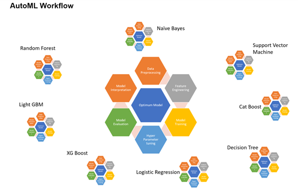
Identifying the model that best fits the data takes time, effort, and expertise in the ML process. The Train Using AutoML tool automates this workflow and identifies the best algorithm with the best set of hyperparameters that fit the data. This implementation is built on an open source implementation called mljar-supervised. The sections below describe each of the steps in the ML process.

Train Using AutoML tool workflow

The Train Using AutoML tool automates the following:

1. Data preprocessing—Successful ML projects require collection of high-quality input data that addresses a specific problem. This data may come from disparate data sources and may need to be combined. Once the data has been collected and synthesized, it must be cleaned and de-noised to ensure that ML algorithms can effectively be trained on it and learn from it. This step is typically time-consuming and tedious, and may require detailed, domain-specific knowledge and experience. Data cleaning can involve identifying and handling missing values, detecting outliers, correcting mislabeled data, and so on, all of which may require a substantial level of time and effort from the ML practitioner. The following are the preprocessing steps:
   1. Remove outliers—Outliers are data points that are dissimilar to the rest of the data points. Reasons for these outliers include data entry errors, data measurement errors, or a legitimate dissimilarity. Regardless of the cause, it is important to remove outliers from the data, as they have a tendency to confuse the model during the training phase. Common methods of addressing outliers are manually correcting the entries or deleting the entries from the dataset.
   2. Impute missing values—Some columns in the dataset may have missing entries. Machine learning models cannot be trained if there are missing entries in the training data. To ensure that there are no missing entries in the dataset, fill the missing entries with valid data using data imputation. Strategies to fill these missing entries include adding the most common occurrence of the value or adding a new value to highlight that the data is missing. For numerical data, one strategy is to use the mean or median of all the entries in the missing data column. Currently, that can be determined by running the Fill Missing Values tool. The Fill Missing Values tool allows you to impute not only with a global statistic from the column but also using spatial strategies such as local neighbors and space-time neighbors, or temporal strategies such as time-series values.
   3. Scale and normalize the data—One of the core assumptions while training a linear model machine learning model such as OLS (the residuals) is that the data being trained is distributed normally; that is, it follows a bell curve.

      

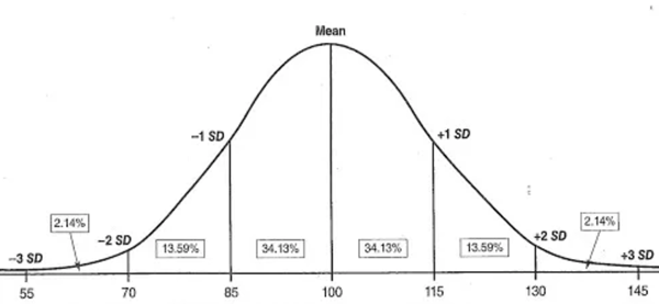
      Before using a linear model, ensure that each column in the dataset is distributed normally. If any columns are not normally distributed, transformations are commonly applied to the data to convert it to a normal distribution.

      Ensure that all columns in the dataset are in the same scale so the model does not give importance to columns whose values fall in the larger scale. This is done by applying scaling techniques on the dataset.

      While the above may be true for linear models, other algorithms such as Logistic regression and the tree-based models—such as Decision Tree, Extra Tree, Random Forest, XGBoost, and LightGBM—don't assume any normality and are more robust to differences in scale, skewed distributions, and so on.

   4. Convert categorical data to numerical—Most of the machine learning models require the data that is being used for training to be in the form of numbers. They cannot work with other data types. Convert nonnumeric columns such as State, Country, City, or Land cover category, Construction type, Dominant political party, and so on, to numbers. Techniques used to convert categorical data to numbers include label encoding and one-hot encoding.
   5. AutoML also provides the capability to use multimodal data for modeling, integrating images and text with tabular data. Multimodal data modeling can help extract insights from diverse data sources. Traditional models often rely on a single type of data, limiting their capacity to fully capture the complexities of real-world phenomena. The newly implemented multimodal, or mixed data, modeling combines the strengths of images, text, and tabular data to provide deeper insights and improve predictive performance. First, features are extracted and processed from each modality using text and image embeddings. Then, they are concatenated with the tabular features to form a unified feature vector for each sample. The concatenated feature vector is typically normalized to ensure that features from different modalities have a similar scale. This combined feature vector containing text embeddings, image embeddings, and tabular features, serves as input to the multimodal model. Images can be used by using the Add Image Attachments parameter in the Train Using AutoML tool.
2. Feature engineering and feature selection—The columns that are used during the model training process are called features. The usefulness of these features while the model learns varies. Some of the features may not be useful, and in these cases, the model improves when the features are removed from the dataset.

   Approaches such as recursive feature elimination and random feature techniques help determine the usefulness of features in the dataset, and features that are not useful in such approaches are generally removed.

   In some instances, combining multiple features into a single feature improves the model. This process is called feature engineering.

   Apart from the new features obtained by combining multiple features from the input, the tool also creates spatial features with names from zone3_id through zone7_id when the Advanced option is used. These new features are generated by assigning the location of input training features to multiple (up to five) spatial grids of varying sizes and using the grid IDs as categorical independent variables named zone3_id through zone7_id. This provides relevant spatial information to the models and helps them learn more from the available data.

3. Model training and model selection—In the model training step, the ML practitioner chooses the appropriate ML algorithm based on the problem and the characteristics of the data. They then begin the iterative process of training models to fit to the data, which often includes experimenting with several ML algorithms. Each of these algorithms may have many different hyperparameters, which are values specified manually by the ML practitioner that control how the model learns. The hyperparameters are then tuned (adjusted) in an effort to improve the performance of the algorithm and achieve better results. This is an iterative process that requires the time and expertise of the ML practitioner. The various algorithms or the statistical models include Linear regression and Logistic regression, other machine learning models such as Decision Trees, Random Forests, and the more recent boosting models such as LightGBM and XGBoost. Although LightGBM and XGBoost outperform most of the other models on almost all datasets, it is difficult to predict which models will work well on a given dataset, so you must try all of the models to compare their performance before deciding on the model that best fits the data. The best fitting model could be identified from its model metric. Different model metrics are returned after training regression and classification models running the Train Using AutoML tool. For some of these metrics, a higher value indicates a better model and for others, a lower value indicates a better model. This is summarized in the following table:

   Model	Low value (best model)	High value (best model)
   Regression	MSE, RMSE, MAE, MAPE	R2, Spearman, Pearson scores
   Classification	Logloss	AUC, F1

   In most cases, combining multiple models into one and taking the output from this combined model outperforms the result from a single model. This step is called model ensembling.

4. Hyperparameter tuning—Although most of the previous steps are iterative, the step that is often the most difficult while training machine learning models is hyperparameter tuning.

   Hyperparameters can be considered as levers that come with each model. The hyperparameters that are used in training a Random Forest model are different from those that are used to train a LightGBM model. Learning about these hyperparameters will help you understand the model.

5. Model selection—The final step in the ML workflow is model evaluation, where you validate that the trained and tuned ML algorithm will generalize well to data that it was not fitted on. This unseen data is often referred to as the validation or test set and is kept separate from the remainder of data that is used to train the model. The goal of this final step is to ensure that the ML algorithm produces acceptable predictive accuracy on new data.

In the ML workflow, there are varying degrees of human input, decision making, and choice occurring at every step.

• Was the appropriate data collected to address the problem and is there enough of it?
• What signifies an outlier in the context of the data?
• If missing values are found, what should replace them?
• Which features should be included in the ML model?
• Which ML algorithm should be used?
• What is an acceptable level of performance for the model?
• What is the best combination of hyperparameters for a model?

This last decision can potentially involve hundreds or even thousands of combinations of hyperparameters that can be iterated. Add a few different feature engineering scenarios and the training and tuning of several different ML algorithms, and the process may become unmanageable and unproductive. Additionally, several of the steps in the ML workflow require expert technical understanding of data science techniques, statistics, and machine learning algorithms. Because of this, designing and running ML projects can be time consuming, labor intensive, costly, and often dependent on trained ML practitioners and data scientists.

In the past decade, machine learning has experienced rapid growth in both the range of applications it is applied to and the amount of new research produced about it. Some of the driving forces behind this growth are the maturity of the ML algorithms and methods, the generation and proliferation of volumes of data for the algorithms to learn from, the inexpensive computers to run the algorithms, and the increasing awareness among businesses that ML algorithms can address complex data structures and problems.

Many organizations want to use ML to take advantage of their data and derive insights from it, but there is an imbalance between the number of potential ML applications and the amount of trained, expert ML practitioners to address them. As a result, there is an increasing demand to standardize ML across organizations by creating tools that make ML widely accessible throughout an organization and can be used off the shelf by non-ML experts and domain experts.

Recently, Automated Machine Learning (AutoML) has emerged as way to address the demand for ML in organizations across all experience and skill levels. AutoML aims to create a single system to automate (in other words, remove human input from) as much of the ML workflow as possible, including data preparation, feature engineering, model selection, hyperparameter tuning, and model evaluation. In doing so, it can be beneficial to nonexperts by lowering the barrier of entry into ML, but also to trained ML practitioners by eliminating some of the most tedious and time-consuming steps in the ML workflow.

AutoML for those who are not ML expert (GIS analysts, business analysts, or data analysts who are domain experts)—The main advantage of using AutoML is that it eliminates some of the steps in the ML workflow that require the most technical expertise and understanding. Analysts who are domain experts can define their business problem and collect the appropriate data, and have the computer do the rest. They don’t need a detailed understanding of data science techniques for data cleaning and feature engineering, they don’t need to know what all the ML algorithms do, and they don’t need to spend time exploring different algorithms and hyperparameter configurations. Instead, these analysts can focus on applying their domain expertise to a specific business problem or domain application. Additionally, they can be less dependent on trained data scientists and ML engineers in their organization because they can build and use advanced models on their own, often without any coding experience required.

AutoML for the ML expert (data scientists or ML engineers)—AutoML can also be beneficial to ML experts. Using AutoML, ML experts do not have to spend as much time supporting the domain experts in their organization and can focus on their own advanced ML work. AutoML can also be a time saver and productivity booster. Many of the time-consuming steps in the ML workflow—such as data cleaning, feature engineering, model selection, and hyperparameter tuning—can be automated. The time saved by automating these repetitive, exploratory steps can be shifted to more advanced technical tasks or to tasks that require more human input (for example, collaborating with domain experts, understanding the business problem, or interpreting the ML results).

AutoML can also help boost the productivity of ML practitioners because it eliminates some of the subjective choice and experimentation involved in the ML workflow. For example, an ML practitioner approaching a new project may have the training and expertise to guide them on which new features to construct, which ML algorithm might be the best for a particular problem, and which hyperparameters are most optimal. However, they may overlook the construction of certain new features or fail to try all the possible combinations of hyperparameters while they are performing the ML workflow. Additionally, the ML practitioner may bias the feature selection process or choice of algorithm because they prefer a particular ML algorithm based on their previous work or its success in other ML applications. In reality, no single ML algorithm performs best on all datasets; some ML algorithms are more sensitive than others to the selection of hyperparameters, and many business problems have varying degrees of complexity and requirements for interpretability from the ML algorithms used to solve them. AutoML can help reduce some of this human bias by applying many different ML algorithms to the same dataset and then determining which one performs best.

For the ML practitioner, AutoML can also serve as an initial starting point or benchmark in an ML project. They can use it to automatically develop a baseline model for a dataset, which can give them preliminary insights into a particular problem. They may decide to add or remove specific features from the input dataset or focus on a specific ML algorithm and fine-tune its hyperparameters. In this sense, AutoML can be viewed as a means of narrowing the set of initial choices for a trained ML practitioner, so they can focus on improving the performance of the ML system overall. This is a commonly used workflow in which ML experts develop a data-driven benchmark using AutoML and build on this benchmark by incorporating their expertise to refine the results.

Standardizing ML using AutoML in an organization allows domain experts to focus their attention on the business problem and obtain actionable results, allows more analysts to build better models, and can reduce the number of ML experts that the organization needs. It can also help boost the productivity of trained ML practitioners and data scientists, allowing them to focus on the multitude of other tasks where it is needed most.

Identify the best model

To identify the best model using the Train Using AutoML tool, complete the following steps:

1. Run simple algorithms, such as Decision Tree (a simple tree with a maximum depth of 4) and linear models.

   This allows a quick examination of the data as well as the results to expect.

2. Train the selected models from the previous step with default parameters. Run the data through a set of more complex algorithms using only the default hyperparameters.

   One model fit is attempted for each algorithm and for all the algorithms available. The available algorithms are Linear, Random Forest, XGBoost, LightGBM, Decision Tree, and Extra Tree.

3. Conduct a random search over the hyperparameter space of each algorithm to find the optimal set of hyperparameters.
4. Construct new features using Golden Features. Determine which of the new features have predictive power, and add them to the original dataset.

   The best set of hyperparameters identified in the previous step are used in this step.

5. Use the optimal set of hyperparameters determined in step 4 to train one best-performing model for each algorithm, and determine the least important features and remove them.

   The results from the best models trained so far are combined. Then the models are stacked and the results of the best models (including stacked) are combined.

Create an ensemble

An ensemble is a collection of models whose predictions are combined by weighted averaging or voting.

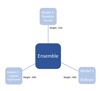
The most common strategies for creating an ensemble are bagging (Random Forest is an example of bagging) and boosting (XGBoost is an example of boosting), which combine the outputs from the models belonging to the same algorithms. Recent techniques, such as those mentioned in Ensemble Selection from Libraries of Models (Caruana et. al 2004) combine diverse models.

To create an ensemble, complete the following steps:

Prerequisite:

Start with the empty ensemble.

1. Add the model in the library that maximizes the ensemble’s performance to the error metric on a validation set.
2. Repeat the previous step for a fixed number of iterations or until all the models have been added.
3. Return the ensemble from the nested set of ensembles that has maximum performance on the validation set.

Model stacking involves combining the results of multiple models and deriving the result from it.

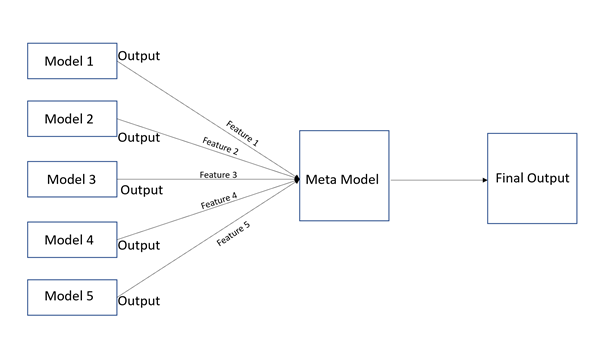
While ensemble approaches combine the results of various models by applying different weights to the outputs, stacking uses the outputs of each base model as features and adds them to a higher-level model: a meta model. The output from the higher-level meta model is used as the final output.

To improve performance, you can create model stacks and combine their outputs to form an ensemble stack.

Interpret the output reports

The Train Using AutoML tool can generate an HTML report as an output.

The main page of the report shows the leaderboard. The same information is also available in the tool output window.

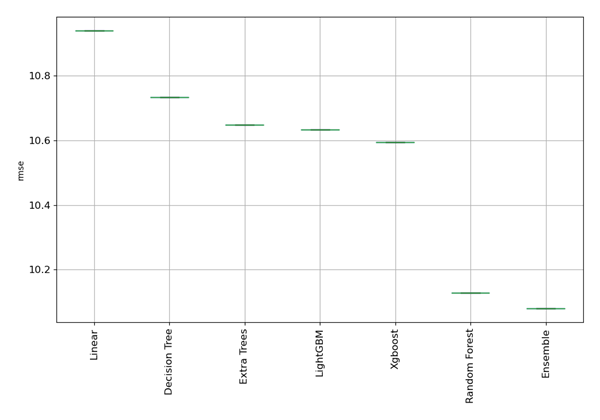
The leaderboard shows the evaluated models and their metric value. For the regression problem, the model with the least RMSE is considered the best model (in this case, the ensemble model). It will be different (for example, logloss) for classification problems.

The AutoML performance box plot below compares the evaluation metric of different models with an evaluation metric (RMSE) on the y-axis and models on the x-axis, as shown below. The box plot shows that the best model is the ensemble model that has the lowest RMSE.

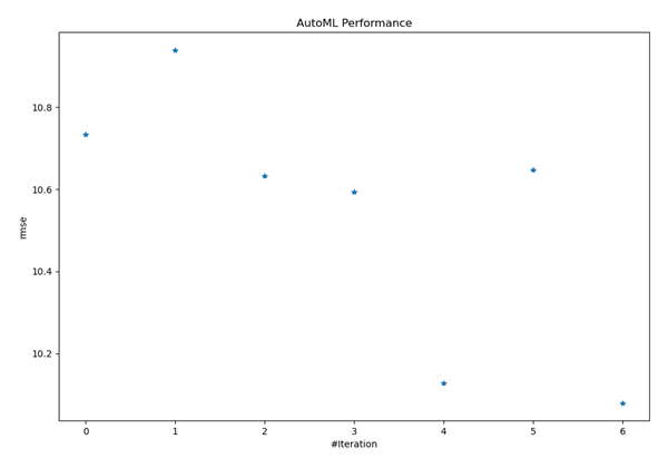
The AutoML performance chart below shows how the evaluation metric for the best performing model, which in this case is the ensemble model, varies across different iterations. The iteration chart can help you understand how consistent the model is across different runs of the model.

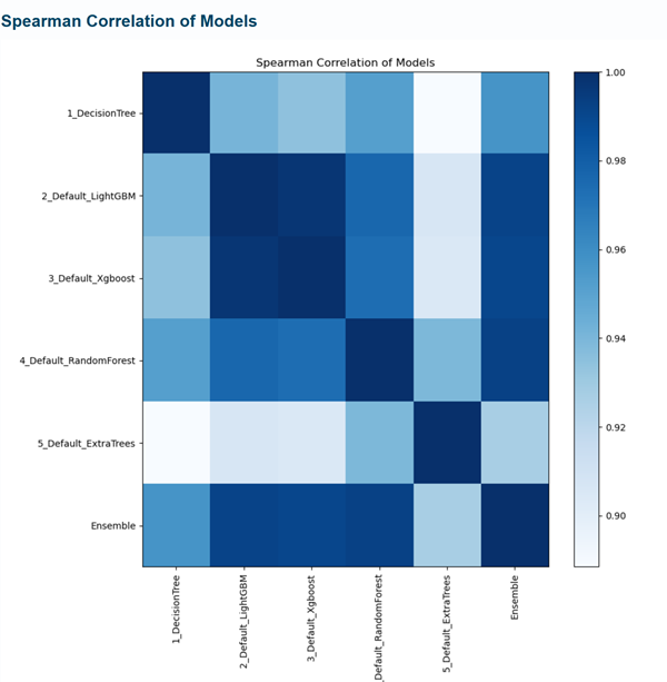
The Spearman correlation shown below is generated for all the models that were evaluated, and the models that are more closely related are shown in darker shades of blue. For example, the outputs from LightGBM and XGBoost are the most closely related (this is expected, as both are boosting algorithms). The output from LightGBM resembles the output from Random Forest compared to the output from Extra Trees.

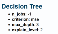
From the leaderboard, you can click the link for any of the models in the Name column to go a page that shows the hyperparameters that were finalized for the model training after completing hyperparameter tuning. In this example, the decision tree was trained with the max_depth value of 3.

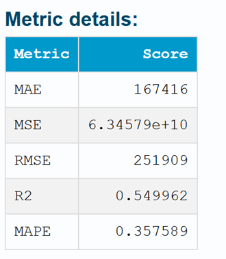
The same page also shows other metrics apart from the one that was used for evaluation. In the example below, which was a regression task, the MAE, MSE, RMSE, R2, and MAPE metrics were used for model evaluation.

The scatter plot of actual and predicted outputs (for a sample of 5,000 data points) is also shown.

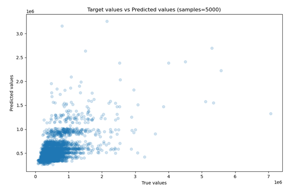
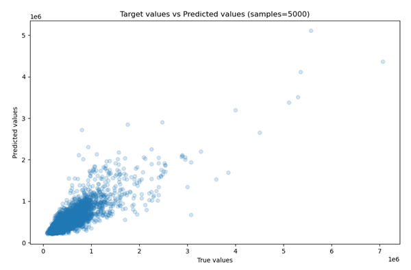
You can use this chart to determine the performance of the model. The figures above show the comparison of the scatter plots of two models obtained from the report. The second model is performing better than the first, where the predicted and true values diverge more.

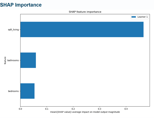
To make models more explainable, the importance of each variable in the final model is also included in the report (similar to feature importance in sklearn). Unlike sklearn, this plot can be generated for nontree models of sklearn as well. This capability of model explanation for models that are not tree based is offered by SHapley Additive exPlanations (SHAP).

SHAP is a game theoretic approach to explain the output of any machine learning model. It connects optimal credit allocation with local explanations using the classic Shapley values from game theory and their related extensions. Details about SHAP and its implementation are available in the SHAP GitHub folder. SHAP output is available only with the Basic option.

In the chart below, you can visualize the global impact of each variable in the housing dataset on the trained model. This demonstrates that the sqft_living feature influences the model the most and is the most important feature, followed by number of bathrooms and bedrooms while predicting the house prices.

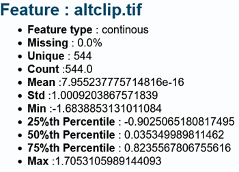
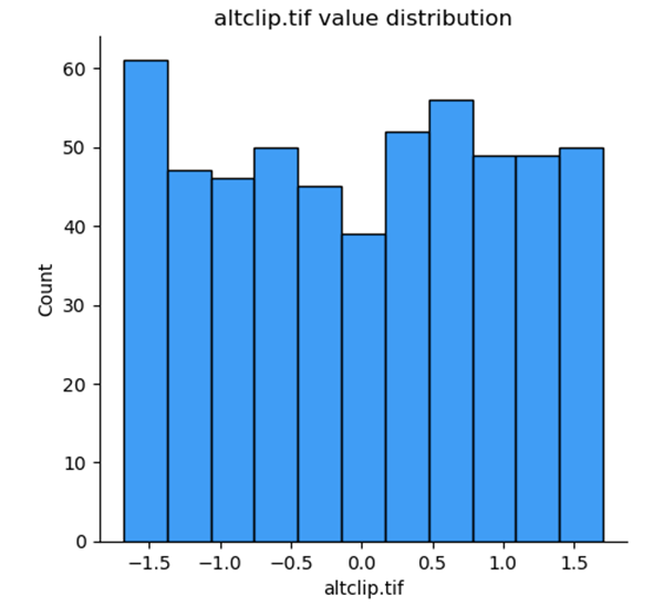
With the Basic option, you also have the option to see the automatic exploratory data analysis report (EDA report), which prints summary statistics for the target variable and the predictors used in model training. The following is a sample EDA report for a variable named altclip.tif:

Predict Using AutoML tool

The Predict Using AutoML tool predicts continuous variables (regression) or categorical variables (classification) on unseen compatible datasets using a trained DLPK model produced by the Train Using AutoML tool.

The input is an Esri model definition file (.emd) or a deep learning package file (.dlpk), which can be created using the Train Using AutoML tool.

Some of the optional outputs that are generated by the Predict Using AutoML tool, in addition to the prediction, are defined by the following parameters and field:

• Get explanation for every prediction—This parameter is used to estimate local variable importance and is useful for understanding a model at a local scale. When the parameter is checked, local variable importance is generated for all explanatory variables including explanatory features, explanatory rasters, and explanatory distance features. A percentage score is added for the explanatory variables representing local variable importance for the predicted values at the respective location to the Output Prediction Features parameter value. For example, if predictors named var1, var2, and var3 are used to train the model—which can be a feature variable, a raster, or a distance variable—fields named var1_imp, var2_imp, and var3_imp are added for each sample in the Output Prediction Features value:

  var1_imp	var2_imp	var3_imp
  0.26	0.34	0.40
  0.75	0.15	0.10

  The variable importance will show the varying importance of each predictor by location, which will also reveal the strength and weakness of each predictor contributing to the local predictions. This parameter is active when the Prediction Type parameter is specified as Predict feature.

• Confidence Score—This score shows the confidence level of the model for the predicted class returned by the model. This is available only for a classification problem, and a prediction_confidence field will be added to the output attribute table displaying score values ranging from 0 to 1, representing low to high probability of the correct class. This field can help identify more confident predictions and less confident predictions.

References

Caruana, Rich, Alexandru Niculescu-Mizil, Geoff Crew, and Alex Ksikes. 2004 "Ensemble Selection from Libraries of Models." Proceedings of the 21st International Conference on Machine Learning. Banff, Canada.Ensemble Selection from Libraries of Models .