Building shell extraction from aerial lidar

This document presents a workflow used to extract building shells (exteriors) from classified aerial lidar. The approach clusters rooftop points into different roof parts, makes a triangulated irregular network (TIN) for each part, extrudes each part’s boundary to the ground, and writes the output to a multipatch feature class. The multipatch-based representation of building exteriors can then be used for visualization and analysis.

An example set of building shells are extracted for an urban area.

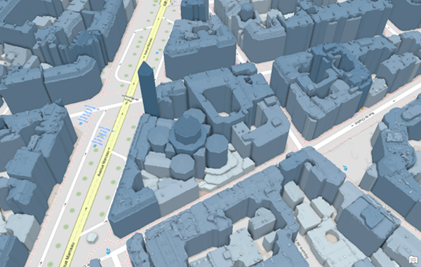
The benefit of this approach is positional accuracy of the rooftops, since they are made directly from the lidar points. It can also model some unusual and unique rooftop forms, as it isn't restricted to a limited set of typical roof forms. Disadvantages include noisy results when viewed up close, interior building corners that are rounded rather than sharp, a potentially output higher vertex count, and lack of multiple levels of detail.

There are other approaches for building shell extraction. One, for example, splits rooftops into different parts, predicts a roof type and eave height for each, and procedurally generates geometry for the part, writing the output to a multipatch feature class. The benefit of this approach is clean and simple geometry. The downside mostly pertains to the question of positional accuracy. The modeled rooftop might not match the actual rooftop very well, though there are ways to identify problematic buildings and fix them. For more information, see the 3D Buildings solution.

Standard roof types and examples using a procedural approach are shown.

Both approaches extrude from the roof/eave edge to down to the ground, so the building sides are simple and vertical. Balconies and overhangs aren't captured in the models.

Requirements:

• ArcGIS Pro 3.3 or later
• Building rooftop classified aerial lidar
• A point density that's at least 4 ppm / 0.5 m spacing
• A raster digital elevation model (DEM) to supply ground height

Concepts

This approach uses rooftop points to form building shell geometry. Clutter on top of the roof, such as antennae, pipes, vents, fans, and other HVAC-related equipment, can be undesirable. Buildings' sides tend to introduce negative consequences coming from things such as balconies and parts that stick out from the side of tall buildings. Therefore, the points classified as building should include the roof but exclude undesirable clutter and building side points.

Rooftop points are clustered based on 3D distance. This separates rooftop parts that are at distinctly different heights from one another. Vertical walls will be dropped between them.

.

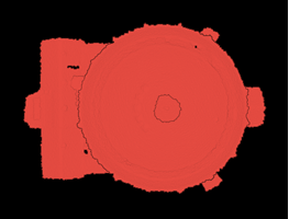
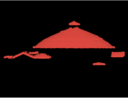
The distance-based clustering is most useful for larger structures in urban areas because they’re more likely to have parts at distinctly different heights. Rooftops with parts that meet one another at common junctures, as is more common with single-family residential homes, will not end up in different clusters.

A cross-sectional view of roof points with different sections that meet each other is shown. Consequently, they will combine into one roof cluster.

The 2D boundary of each cluster is used as a roof part and is extruded to the ground, forming the walls of the building shell. Cluster boundary polygons, which are concave hulls, are defined using a concept called alpha shapes. A key parameter that defines how tight the boundary is fit around the cluster is called the alpha radius.

From left to right, a top-down view of a point set for a portion of a building, a corresponding portion of an output roof polygon made with an alpha radius of 0.5m, and a result using an alpha radius of 1.0m. Note how certain corners are sharper with the smaller alpha radius, while the building sides are cleaner using the larger value.

The different cluster boundaries for a building do not meet cleanly and this is arguably a weakness of the approach, as there are gaps between parts. This isn’t much of a problem except when viewing from a close distance.

A top-down view of rooftop part polygons for a building is shown on the left and the corresponding building shell, in perspective, on the right.

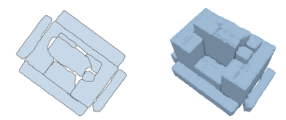
While this approach to building shell modeling has its limitations, the results can often be sufficient for the job and provide for closer approximation than techniques that rely on modeling based on roof types.

Workflow

The workflow starts out using the Extract Objects From Point Cloud geoprocessing tool. This tool extracts bounding geometries around clusters of like-classified points. Use this tool to get a 2D footprint for each roof part, and for each part, the z range of the points that formed it. The tool then uses those roof polygons as input to the LAS Building Multipatch geoprocessing tool. It builds a TIN for each part using building classified points that are also filtered by the height range associated with the roof part, and extruding the TIN boundary down to the ground.

Note:

To save time, experiment on a representative subset to get an idea what a good set of parameter values will be with your data before applying to a larger collection.

Parameters for the Extract Objects From Point Cloud geoprocessing tool

1. Input Point Cloud—The input LAS dataset.
2. Class Codes to Extract—Indicate which class code represents the rooftop points. It’s generally class 6. You can default the output Group ID to be the same.
3. Output Object Features—The output feature class.
4. Output Geometry Type—The 2D concave hull.
5. Clustering Distance—This will be the distance of separation in Z between clusters. Values in the range of 0.5 to 3.0 meters are reasonable. Try starting at 1.5 meters. The intention is for points that belong to a rooftop part to be within that distance of each other, and thus be clustered as a group, while different roof parts will be a larger distance away and thus get clustered separately.
6. Vertical Clustering Scale factor—Start with a value of 1.0. Using a larger value will exaggerate the impact of height difference between points while a smaller value will decrease it. When using a value of 0.0, height no longer applies and the clustering is done in 2D. Use 0.0 to get the building footprint as opposed to rooftop part prints.
7. Calculate a Unique Radius For Each Object—Leave this parameter off by default, but it's worth experimenting with. If you turn it on, you’re likely to get a more detailed boundary of each object. While potentially beneficial, it can also introduce more noisy building side walls.
8. Alpha Radius—This parameter controls how closely the boundaries of the output polygons are fit around the point clusters and it is enabled when the previous parameter is off. Smaller values yield more detail along walls and around interior building corners, while larger values generalize more, yielding smoother walls. Try starting with 2 meters.
9. Minimum Number Of Point—Leave this parameter at a default of 10 unless you either require larger clusters (increase the value) or want to allow for smaller clusters (decrease the value).

Review the results. While you can display the polygons in a 2D map, you might not see polygons that are covered by other polygons. Set the symbol fill to transparent, leaving just the outlines, to see the otherwise hidden polygons. For a different, and arguably better view, you can use a local 3D scene to display the polygons in 3D (using the MIN_Z or MAX_Z attribute added to the output feature class).

You should consider deleting polygons with small 2D areas because these are mostly noise and they add unnecessary computational expense for rendering and analysis. You can do this using a combination of the Select Layer By Attribute tool followed by Delete Features. As a starting point, try 6.0 square meters as a cutoff size (this is the default minimum area used by the Classify LAS Building tool).

You should also consider removing holes in polygons. Many holes are made because one higher roof part is in the middle of a lower roof part. Closing the lower part’s hole will create a cleaner appearance when the upper part gets extruded through it. There is the risk of removing holes that should remain though (for example, ones that don’t have other parts extruded through them), so do this with care. You can use Eliminate Polygon Part with the Eliminate contained parts only option. An area of 25 square meters is a reasonable starting point.

Parameters for the LAS Building Multipatch geoprocessing tool

1. Input Features—Use the roof part polygons that were output by the Extract Objects From Point Cloud geoprocessing tool.
2. LAS Rooftop Point Selection—Indicate what points to use for rooftops. If you select Building Classified Points, the tool will use class 6 points. If your data uses a different class code, or codes, for rooftop points, assign a layer filter using the correct code or codes and select the Layer Filtered Points option.
3. Sampling Resolution—This bins the rooftop points and uses the highest point in each bin. We’re making a TIN from these points and the triangulation for this TIN is 2D. It doesn’t support truly vertical faces or overhangs. Your rooftop classified points might contain different roof parts that overlap one another.
4. Ground Height—The roof part boundaries are extruded down to the ground. This parameter allows you to pick a DEM or attribute from the polygons to get the ground height. One way polygons can get that attribution is through use of the Add Surface Information tool. The benefit of using a height attribute over a DEM is that, while it has some cost to calculate, the information can be reused repeatedly without cost. When using a DEM as input, the calculation to find the ground height from the DEM is repeated each time you rerun the tool.
5. Output Multipatch Feature Class—The output building shells.
6. Simplification Tolerance—Before a rooftop TIN is converted to a multipatch, it can be generalized to reduce the number of nodes. This is desirable for the sake of performance downstream. The tolerance is the height difference allowed between the generalized TIN and the original. Consider using a value equal to the vertical accuracy of the lidar (for example, 10 cm).
7. Minimum Height Field—This references an attribute in the input polygon feature class and is used as a filter. Only points equal to or higher than this (and inside the polygon) will be used. This filters out data from clusters that may be above or below the cluster that generated the polygon. Specify the MIN_Z field that was output from the Extract tool.
8. Maximum Height Field—This references an attribute in the input polygon feature class and is used as a filter. Only points equal to or lower than this (and inside the polygon) will be used. This filters out data from clusters that may be above or below the cluster that generated the polygon. Specify the MIN_Z field that was output from the Extract tool.

If your data has buildings classified in a way that includes rooftop clutter and building side points, and this is causing problems, try making a copy of a test area, and, as an experiment, redo the building classification using the Change LAS Class Codes geoprocessing tool to reset the building class to 1 followed by the Classify LAS Building geoprocessing tool.

Experiment with Classify points above the roof in the multipatches. The Classify LAS Building geoprocessing tool has an option to place above roof points into class 6 or another class. It’s most flexible to place them in a custom class and optionally include them with the Extract Objects From Point Cloud geoprocessing tool.

This tool allows you to use input multiple classes and treat them as one by assigning them the same output Group ID. The points with the same Group ID will be treated as the same class for the sake of clustering. If you include above roof points with the Extract Objects From Point Cloud geoprocessing tool, it makes sense to include them with the LAS Building Multipatch geoprocessing tool. You would do this by turning on only the building and above roof points in the LAS dataset layer then choosing to use layer filtered points with the tool. You can also treat above roof as its own class to extract. Keeping these separate from the other parts of the roof will make them visually more distinct because they will have vertical sides. You’ll also be able to turn them on and off independently of the other building parts.

Try using 3D layer properties and extrusion to display extracted rooftop part polygons. Without the lidar points, these will have flat tops, but all displayed in combination can look reasonable from a distance and rendering-efficient because of their relatively low vertex count. A side benefit of using Add Surface Information between the extracted roof part polygons and a DEM, to add the ground height as an attribute to the polygons, is you can then calculate building height relative to the ground (the roof part polygons will already have a MAX_Z that came from the point clusters) and use that to symbolize building parts.

Lidar data source acknowledgements:

• Graphics 1, 3: French National Institute of Geographic and Forestry Information
• Graphics 4, 7: The Netherlands Rijkswaterstaat, Ministry of Infrastructure and Water Management
• Graphic 5: USGS Lidar Central Eastern Massachusetts