The Assess Sensitivity to Attribute Uncertainty tool evaluates how the analysis results of select tools in the Spatial Statistics toolbox change when the values of one or more analysis variables (attributes) are uncertain. Attribute uncertainty can be specified using margins of error, upper and lower bounds, or a specified percentage of the original value. This tool accepts the output features from the following tools:
- Hot Spot Analysis (Getis-Ord Gi*)
- Optimized Hot Spot Analysis
- Cluster and Outlier Analysis (Anselin Local Moran's I)
- Optimized Outlier Analysis
- Generalized Linear Regression
- Spatial Autocorrelation (Global Moran's I)
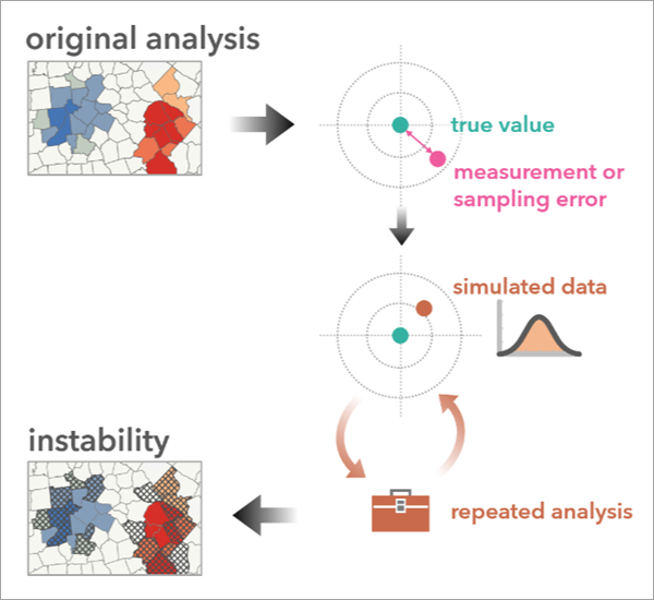
The tool performs a sensitivity analysis by repeatedly simulating new data using the original analysis variable and its measure of uncertainty. It then reruns the original analysis tool many times using the simulated data and summarizes the results. If the results of the simulations closely resemble the original results, this gives you confidence that the original results are robust and reliable. However, if the simulations produce large differences from the original results, you should be more hesitant to make strong conclusions from the original results.
Potential applications
Potential applications of the tool include the following:
- A local charitable organization uses hot spot analysis to prioritize areas within the county for services to reduce poverty. They plan to focus on regions where the analysis indicates high clustering and intensity of poverty (hot spots with 99% confidence). Monitoring how the hot spots change may lead to reinforcing or reconsidering their service priorities.
- A large retail chain has developed a generalized linear regression model to estimate how demographic factors such as age and disposable income influence sporting goods sales. The explanatory variables collected through surveys include both upper and lower bounds. By incorporating the uncertainty in these variables, the retailer can explore the potential range in sales volume.
Attribute uncertainty
Attribute uncertainty is the variability in data values that stems from natural and unavoidable aspects of data collection and aggregation, such as sampling error or measurement error. Sampling errors occur when data is collected from a subset of a population, introducing questions about how well the sample represents the entire population. Measurement error arises when a data collection instrument, such as a thermometer or wind meter, introduces minor variations in the recorded values compared to the true values. Data is often provided with the best estimate of the true value of the measurement, called the point estimate, and some measure of its level of uncertainty. While these sources of uncertainty can affect the precision of the data, they are present in any real-world data collection process. Recognizing and exploring attribute uncertainty and its impact on analytical results can help make analyses more transparent and robust.
How uncertainty is quantified
This tool supports three ways to specify attribute uncertainty: margin of error, upper and lower bounds, and a percentage above and below an attribute value.
Margin of error
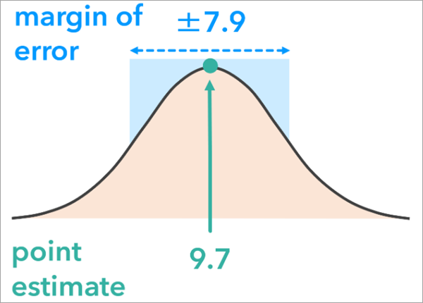
A margin of error represents the range within which the attribute’s true value will likely fall. It is associated with a confidence level (such as 90 percent), indicating how confident you can be that the attribute’s actual value lies within the range defined by the estimate, plus or minus the margin of error. For example, a survey may estimate that a county has 2,500 people in poverty, with a margin of error of 300 at the 90 percent confidence level. This means you can be 90 percent confident that the true number of people in poverty is between 2,200 and 2,800. When using this method, a margin of error field is required for at least one analysis variable. This field contains the numeric error bound representing how far above or below the sample estimate the true population value is expected to fall. The confidence level is 90 percent by default and can be adjusted using the Margin of Error Confidence Level parameter.
Note:
Margins of error are typically recorded as fields alongside the original variable. This is the case with many variables in the ArcGIS Living Atlas of the World data sourced from the U.S. Census Bureau’s American Community Survey (ACS). Many national statistics organizations provide similar measures of uncertainty.
Upper and lower bounds
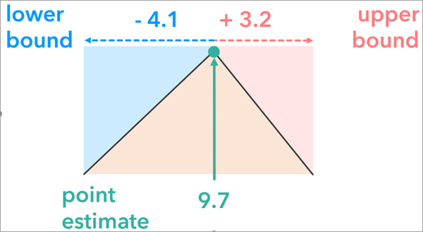
Upper and lower bounds represent the uncertainty of an attribute by explicitly specifying a range around an estimate. Unlike the margin of error, upper and lower bounds do not need to be symmetrical around the point estimate.
Percent below and above
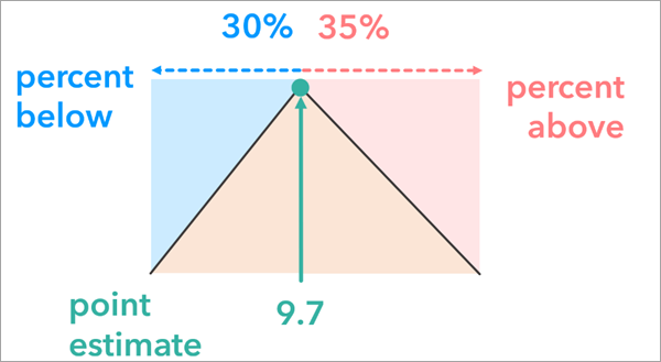
The percent below and above option represents attribute uncertainty by adjusting the original attribute value of each feature by a specified percentage. This creates a range around the estimate that may contain the true value. This approach can be useful when other methods, such as margin of error or upper and lower bounds, are not available to express uncertainty.
Note:
Unlike the margin of error and upper and lower bound options, which allow attribute uncertainty to be specified differently for each feature, the percent below and above option applies the same definition of uncertainty to all features.
Using simulations to address uncertainty
To evaluate how sensitive the analysis results are to uncertainty, the tool generates simulated datasets based on the original analysis variable and its measure of uncertainty. Ideally, each simulated dataset represents a plausible version of the data that might exist in the real world. In addition, there are different assumptions about how the true value might be centered around or spread from the point estimate. The tool uses probability distributions to restrict the simulated data values to capture the range and the likelihood of different realizations of the data. Three distributions are supported: normal, triangular, and uniform. When simulating data for Generalized Linear Regression, the correlation structure between the explanatory variables is maintained. For analysis results from other tools, data is simulated independently from each feature. To account for the dependence among the explanatory variables, their correlation is estimated globally and the simulated values for each feature are generated by adding random noise of a multivariate normal distribution with mean zero and covariance matrix based on the global correlation among the explanatory variables. Since the random noise is based on a multivariate normal distribution, simulations for Generalized Linear Regression only support the normal simulation method.
Normal
The Normal option of the Simulation Method parameter is commonly used when a margin of error with an associated confidence level is available. This option uses a normal (or Gaussian) probability distribution with a mean equal to the value of the original analysis variable and a standard deviation based on the feature’s margin of error value and confidence level.
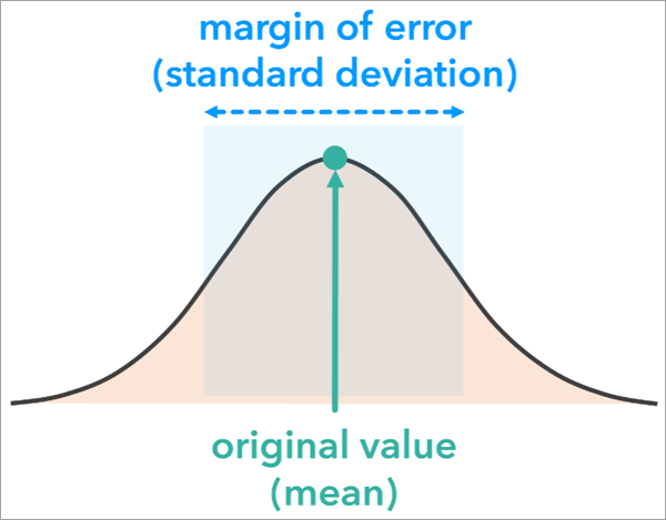
As the shape of the probability distribution suggests, values closer to the original estimate are more likely to be generated than those farther away. However, this can vary significantly depending on the margin of error. Locations with larger margins of error—often due to smaller sample sizes—will have distributions with longer tails, meaning the simulations are more likely to generate values farther from the original estimate.
Triangular
A triangular distribution is commonly used when the original value represents a likely estimate of the true value. The Triangular option of the Simulation Method parameter is particularly useful with asymmetric distributions in which the values are more likely to cluster around the estimated value but with an asymmetric spread. A triangular distribution is constructed and used to simulate data for each feature based on the minimum data value, the feature’s original value, and the maximum data value. The Uncertainty Type parameter value determines the minimum and maximum data values of the triangular distribution.
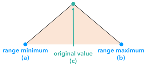
The shape of the triangular probability distribution ensures that values close to the original value are more likely to be generated than values in the extremes of the distribution.
Note:
Unlike the normal distribution, the shape does not need to be symmetrical. For example, the lower and upper bound may differ.
Uniform
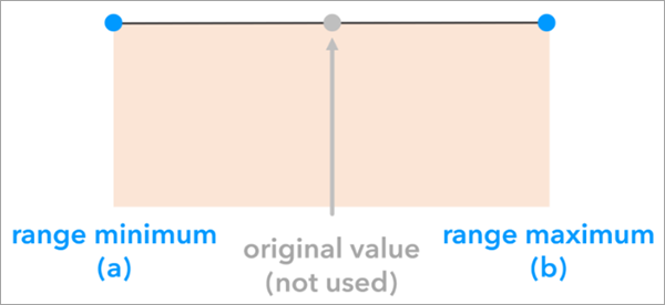
The Uniform option of the Simulation Method parameter is used when the original value at each location is a poor estimate of the true value, and the only available information about attribute uncertainty is the range of possible values. This option uses a uniform probability distribution with two parameters: the minimum in the range set by the uncertainty type, and the maximum in the range set by the uncertainty type. Unlike normal and triangular distributions, the uniform distribution does not use the original value in the probability distribution parameters; each value between the minimum and maximum is equally likely to be generated in the simulations.
Supported tools
Unlike most geoprocessing tools that accept an existing layer as an input, the input to this tool is the result layer from one of the following tools in the Spatial Statistics toolbox:
- Hot Spot Analysis (Getis-Ord Gi*)
- Optimized Hot Spot Analysis
- Cluster and Outlier Analysis (Anselin Local Moran's I)
- Optimized Outlier Analysis
- Generalized Linear Regression
- Spatial Autocorrelation (Global Moran's I)
Hot Spot Analysis, Optimized Hot Spot Analysis, Cluster and Outlier Analysis, and Optimized Outlier Analysis tools
For the Hot Spot Analysis (Getis-Ord Gi*), Optimized Hot Spot Analysis, Cluster and Outlier Analysis (Anselin Local Moran’s I), and Optimized Outlier Analysis tool results, stability is assessed by determining how frequently a feature changed categories in the repeated analysis runs. For example, if a feature was a hot spot with 90 percent confidence in the original analysis and changed to any other category in one of the runs using simulated data, that counts as a category change. The tool counts the number of times a feature’s category changes. Features are marked as unstable if fewer than 80 percent of the simulations resulted in the original category.
The tool produces a group layer containing an instability layer and a copy of the original analysis results.
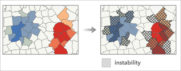
Additionally, the group layer contains a chart displaying the count of features for each original analysis category and each predominant category. The predominant category is the one that occurred most frequently across all of the repeated runs of the tool at each location.
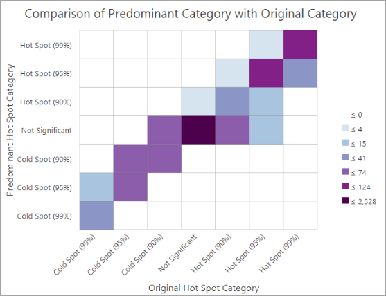
This chart can help identify categorical instability patterns. A perfectly stable result in which each original category perfectly matched the predominant category would fill the cell diagonals.
Note:
The tool does not support analysis results from aggregated points when running the Optimized Hot Spot Analysis or Optimized Outlier Analysis tool.
Generalized Linear Regression tool
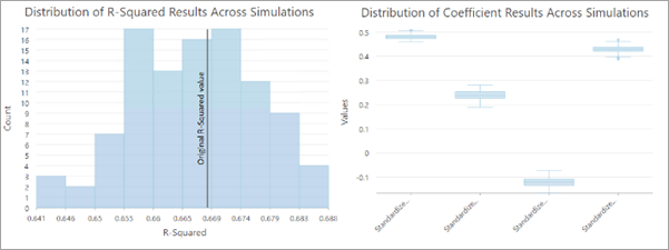
When assessing the uncertainty of a Generalized Linear Regression analysis, the main results of the Generalized Linear Regression tool are charts that display the distribution of regression diagnostics across the simulated runs, such as R-squared and explanatory variable coefficients. The tool provides a group layer containing a copy of the original analysis result, a table summarizing the results from repeated runs of the original tool, and three charts displaying the distribution of R-squared, Jarque-Bera statistical significance, and standardized explanatory variable coefficients.
Spatial Autocorrelation (Global Moran's I) tool
For the Spatial Autocorrelation (Global Moran’s I) tool results, the goal of the tool is to help you understand how certain the original assessment of global spatial autocorrelation would be under attribute uncertainty. The tool provides a group layer with a copy of the original analysis results, a table summarizing the results of repeated runs of the tool, and charts displaying the distribution of Moran’s index values and their z-scores.
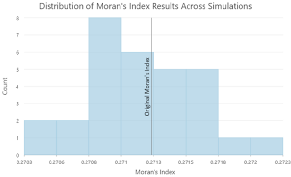
Generally, most of the Moran's index values and their z-scores will be smaller than the original values because adding random uncorrelated noise to data values tends to reduce the spatial autocorrelation of the data.
Note:
The Spatial Autocorrelation (Global Moran’s I) tool does not produce output features. Use the original input features that were used in the Spatial Autocorrelation (Global Moran’s I) tool analysis as the Analysis Result Features parameter value.
Additional considerations
The subsections below provide additional information.
Alter the stability threshold in the output
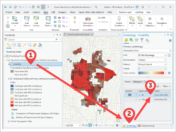
For Hot Spot Analysis (Getis-Ord Gi*), Optimized Hot Spot Analysis, Cluster and Outlier Analysis (Anselin Local Moran’s I), and Optimized Outlier Analysis tool results, the instability layer applies a default stability threshold of 80 percent. This means that for a feature to be considered stable, the feature must result in the same category as the original analysis in more than 80 percent of simulations. Increasing this threshold will designate a higher number of features as unstable, and decreasing this threshold will designate fewer features as unstable.
The threshold that defines stability can be configured using the layer symbology settings. To change the threshold, you must first find and select the instability layer in the output group layer. Second open the Symbology pane, and third double-click the Upper value cell for the 80 percent class and edit the threshold value.
Simulation data limits
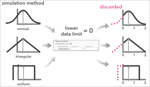
You can set limits on the range of simulated values for an analysis variable. This can be useful when the analysis variable should not be negative (counts) or should have a range between zero and 100 (percentages). Use the Simulation Data Limits parameter to set the range of possible values for each variable. When specifying a Simulation Data Limits parameter value, the tool discards simulated values that result outside of the specified range and repeats the simulation.
Save the intermediate simulation results
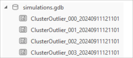
The simulations that the tool creates can be saved as feature classes. Use the Workspace for Simulation Results parameter to set an existing workspace in which the tool will save each simulation result.
The naming convention of each file follows the following format: Name of analysis result features _ Simulation ID _ Simulation Time Stamp. Each simulation result feature class contains the schema of the original analysis result.
The intermediate simulation results may be useful for further analysis. For example, you may examine a workspace of the Generalized Linear Regression tool simulation results to further understand the distribution of predicted values across simulations.
Geoprocessing operations metadata
To find the analysis tool, input features, and additional parameters used in the analysis, the tool reads the metadata from the Analysis Result Features parameter value. Consequently, the analysis that produced the analysis result features must be configured to write to metadata.
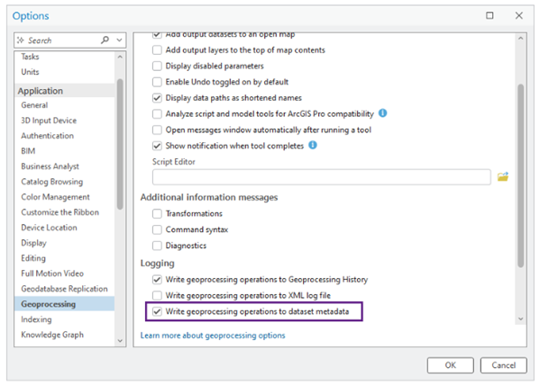
This setting is activated by default. To confirm this setting, open the Options dialog box, click the Geoprocessing tab, and in the Logging section, verify that the Write geoprocessing operations to dataset metadata option is checked.
Note:
The tool does not support Spatial Autocorrelation (Global Moran’s I) tool analyses run on hosted layers since the metadata cannot be modified for these datasets.
Additional resources
For more information, see the following resources:
- JingXiong Zhang and Michael Goodchild. 2002. "Uncertainty in Geographical Information." Taylor & Francis. ISBN 0-203-47132-6. https://doi.org/10.1201/b12624.
- Raphaella Diniz, Pedro O.S. Vaz-de-Melo, Renato Assunção. 2024. “Data augmentation for spatial disease mapping.” Spatial Data Science Symposium 2021 Short Paper Proceedings. https://doi.org/10.25436/E2KS35
- Michele Crosetto and Stefano Tarantola. 2001. "Uncertainty and sensitivity analysis: tools for GIS-based model implementation." International Journal of Geographical Information Science. 15:5, 415-437. https://doi.org/10.1080/13658810110053125
- Zhou Dimin. 2010. “Research on Propagation of Attribute Uncertainty in GIS.” 2010 International Conference on Intelligent Computation Technology and Automation.
- Hyeongmo Koo, Takuya Iwanaga, Barry F.W. Croke, Anthony J. Jakeman, Jing Yang, Hsiao-Hsuan Wang, Xifu Sun, Guonian Lü, Xin Li, Tianxiang Yue, Wenping Yuan, Xintao Liu, and Min Chen. 2020. “Position paper: Sensitivity analysis of spatially distributed environmental models- a pragmatic framework for the exploration of uncertainty sources.” Environmental Modelling and Software. https://doi.org/10.1016/j.envsoft.2020.104857
- Hyeongmo Koo , Yongwan Chun, and Daniel A. Griffith. 2018. “Geovisualizing attribute uncertainty of interval and ratio variables: A framework and an implementation for vector data.” Journal of Visual Languages and Computing 44 89-96. https://doi.org/10.1016/j.jvlc.2017.11.007
- Robert Haining, Daniel A. Grifith, and Robert Bennett. 1983. “Simulating Two-dimensional Autocorrelated Surfaces.” Geographical Analysis. https://doi.org/10.1111/j.1538-4632.1983.tb00785.x
- Sirius Fuller and Charles Gamble. 2020. "Calculating Margins of Error the ACS Way." American Community Survey (ACS) Programs and Surveys, U.S. Census Bureau.
- Shuliang Wang, Wenzhong Shi, Hanning Yuan, and Guoqing Chen. 2005. "Attribute Uncertainty in GIS Data". Fuzzy Systems and Knowledge Discvery Conference. 3614, 614-623. https://doi.org/10.1007/11540007_76
- Ningchuan Xiao, Catherine A. Calder, and Marc P. Armstrong. 2007. "Assessing the effect of attribute uncertainty on the robustness of choropleth mapclassification." International Journal of Geographical Information Science. 21:2, 121-144. https://doi.org/10.1080/13658810600894307