How Bivariate Spatial Association (Lee's L) works

The Bivariate Spatial Association (Lee's L) tool measures the spatial association (dependence) between two continuous analysis variables by calculating the Lee's L statistic. The statistic characterizes the degree of correlation of the variables and their copatterning (the similarity of spatial clustering). The Lee's L statistic will be between -1 and 1 and is conceptually similar to a correlation coefficient but is adjusted to account for spatial autocorrelation of the two variables. Lee's L values close to 1 indicate that the variables are highly positively correlated (when one value is high, the other tends to also be high) and that each variable has high spatial autocorrelation (high and low values of the variables each tend to cluster together). Values close to -1 indicate that the variables are highly negatively correlated (when one value is high, the other tends to be low) and that each variable has high spatial autocorrelation. Values close to 0 indicate that the variables are not spatially associated, meaning that they are either uncorrelated or that they are not spatially autocorrelated. The statistic can also be partitioned locally to each input feature and categorized so you can investigate how the spatial association of the analysis variables changes across a study area.

Accounting for the spatial autocorrelation of the variables is essential for assessing the spatial association between the analysis variables because traditional statistical tests based on Pearson correlation are not valid when the variables are spatially autocorrelated. Additionally, these traditional tests do not assess copatterning of the two variables, which is a critical aspect of the spatial relationship between the variables.

The Lee's L statistic is calculated by combining the correlation of local neighborhood averages of the two analysis variables and adjusting the correlation by spatial smoothing scalars of each analysis variable. The spatial smoothing scalars are values between 0 and 1. Smoothing scalars close to 1 indicate strong spatial autocorrelation (positive or negative), and values close to 0 indicate that the values are spatially random and not autocorrelated. Small spatial smoothing scalars will reduce the Lee's L statistic relative to the Pearson correlation to adjust for the lack of spatial clustering of the variables.

The following images show various examples of maps of two analysis variables and the associated Pearson correlations and Lee's L statistics for the variables. In each image, the blue triangles have the value 1, and the orange triangles have the value 0.

In the first image below, both analysis variables have the same values at each location, so their Pearson correlation is equal to 1. Additionally, they each have high positive spatial autocorrelation with high and low values each clustering together. This results in a Lee's L statistic equal to 0.801, which indicates high positive spatial association between the variables.

In the second image below, the values of the second analysis variable are shifted one triangle to the right so that 30 of the 54 triangles have matching values. This results in a Pearson correlation equal to 0.167. However, because of the strong spatial autocorrelation of each analysis variable, the Lee's L statistic is slightly higher: 0.186. This indicates weak to moderate positive spatial association between the variables.

In the third image below, the values of the second analysis variable are shifted to the other side of the hexagonal study area, and 18 of the 54 triangles have matching values. This results in a Pearson correlation equal to -0.500, and the Lee's L statistic is equal to -0.490, which indicates moderate to strong negative spatial association between the variables.

In the final image below, both analysis variables have negative spatial autocorrelation, and none of the triangles have the same value. This results in a Pearson correlation equal to -1, and the Lee's L statistic is equal to -0.204, which indicates weak to moderate negative spatial association between the variables.

Local Lee's L statistics

The Lee's L statistic can be partitioned to each input feature to see how the spatial association between the variables changes spatially and locally. Some regions or locations may have higher or lower spatial association than the overall (global) Lee's L statistic due to changing local correlations and local spatial smoothing. You can determine whether the local spatial association is higher or lower than the global spatial association by directly comparing the values of local Lee's L statistics to the global Lee's L statistic. Unlike the global statistic, the local statistics can be larger than 1 or less than -1, and the average of the local statistics always equals the global statistic.

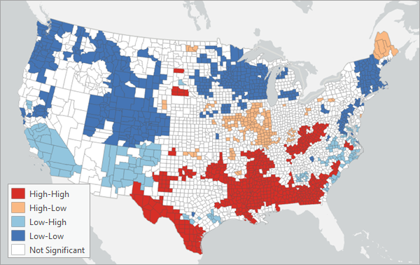
You can also classify the local Lee's L statistics into several categories based on their statistical significance and the values of the neighborhoods of each feature. There are five possible categories for each feature: Not Significant, High-High, High-Low, Low-High, and Low-Low. If the local Lee's L statistic is not at least 90 percent significant for a feature, it will be classified as Not Significant. Otherwise, if the neighborhood average of the first analysis variable is greater than the average of the first analysis variable, and the neighborhood average of the second variable is greater the average of the second variable, it will be classified as High-High. Similarly, if the first variable is less than the average, and the second variable is greater than the average, it will be classified as Low-High (and vice versa). It is important to distinguish these categories because if the two variables are positively spatially associated, it means that low values of the two variables tend to cluster together and high values tend to cluster together. However, both situations will result in large local Lee's L statistics, so the categories clarify whether each feature has high association because both variables are high or because both variables are low. Similarly, for negative spatial association, the classifications clarify whether a feature has a negative local Lee's L statistic because the first variable is high and the second variable is low, or whether the first variable is low and the second variable is high.

When run in an active map, the output feature layer will draw based on these five categories. For positively spatially associated variables (global Lee's L statistic greater than 0), the layer will contain mostly High-High and Low-Low categories. For negatively spatially associated variables (global Lee's L statistic less than 0), the layer will contain mostly High-Low and Low-High categories.

Example use cases

You can use the tool for the following scenarios:

• Investigate the spatial association between education levels and household income in different neighborhoods of a large city. Do areas of higher education correspond to areas of higher household income?
• Research the spatial association between vegetation coverage and air quality. Do areas with more vegetation tend to have better air quality? Is the association statistically significant?
• Is there a relationship between crime rates and property values? Does the relationship change in different regions of a metropolitan area?

Permutations and p-values

You can test the global and local Lee's L statistics for statistical significance using permutations. The permutations randomly reassign all values of the two analysis variables to a new location (keeping the two values paired together at each new location), and the global and local Lee's L statistics are calculated for the permuted values. This process repeats a large number of times (controlled by the value of the Number of Permutations parameter), and this builds reference distributions that can be compared to the original global and local Lee's L statistics. If the original value is on the extremes (right or left) of the reference distribution, it means the original value is unlikely to be the result of a random variation, and the spatial association is statistically significant. The p-value for the global Lee's L statistic is returned as a geoprocessing message, and the p-values and significance levels of the local Lee's L statistics are returned as fields of the output feature class. See the Tool outputs section below for more information.

Note:

The p-values are calculated by counting the number of permuted values that are more extreme than the original value, adding one, and dividing by the number of permutations plus one. This adjustment to the numerator and denominator is made to adjust for small samples and to ensure that the p-values are never equal to zero. The value is then doubled so that the p-value is from a two-sided hypothesis test. The side of the test is determined by the side that has a smaller proportion of more extreme values (permuted values that are greater than or less than the original value). The p-values of the local Lee's L statistics are not adjusted for multiple hypothesis testing, so take that into consideration when interpreting any particular local p-value.

Neighborhood types

The global and local Lee's L statistics require a neighborhood around each feature to estimate the spatial association. You can specify the neighborhood of each feature using the Neighborhood Type parameter. The parameter has the options described below for defining the features that are used as the neighbors of each feature. For all neighborhood types, the feature is included in its own neighborhood.

• Fixed distance band—All features within a specified distance (up to a maximum of 1,000 features) will be used as neighbors. The default distance is the shortest distance that ensures each feature includes at least one additional neighbor. Provide the distance in the Distance Band parameter. For polygons, the distances between centroids will be used to determine neighbors.

  

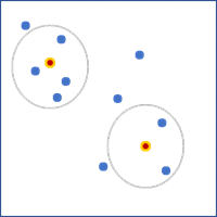
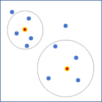
• K nearest neighbors—A fixed number of features closest to the focal feature will be used as neighbors. Provide the value in the Number of Neighbors parameter. This value does not include the feature itself, so the number of features used in the calculations will be one larger than the specified value. For polygons, the distances between centroids will be used to determine neighbors.

  

• Contiguity edges only—Any polygons sharing an edge with the feature will be used as neighbors. This option is only applicable for polygon features.

  

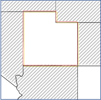
• Contiguity edges corners—Any polygons sharing an edge or corner with the feature will be used as neighbors. This option is only applicable for polygon features.

  

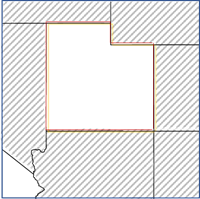
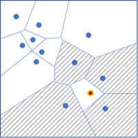
• Delaunay triangulation—Neighbors will be determined by sharing edges or corners in their Delaunay triangulation (Thiessen polygons) clipped to the convex hull of the points. This option is only applicable for point features.

  

• Get spatial weights from file—Neighbors and weights of each feature will be defined by a spatial weights matrix file specified in the Weights Matrix File parameter. You can create the file using the Generate Spatial Weights Matrix or Generate Network Spatial Weights tools.

For distance band and number of neighbors neighborhoods, neighbors closer to the feature can be given higher weights using a kernel function that decreases with distance. To apply larger weights to closer neighbors, specify the Bisquare option for the Local Weighting Scheme parameter.

The bisquare kernel defines weights using the following formula:

The kernel function depends on a bandwidth that controls how quickly the weights diminish with distance. The bandwidth for each kernel is provided in the Kernel Bandwidth parameter. For the k nearest neighbors neighborhood, if you do not provide a bandwidth value, each feature will use a different (adaptive) bandwidth equal to the distance to the (k+1)th neighbor of the feature. For the distance band neighborhood, the kernel bandwidth defaults to the same value as the Distance Band parameter.

Note:

All features will have a weight equal to one for the weight of the feature to itself, even if the spatial weights file does not have these weights assigned. Additionally, the weights for each feature's neighborhood will be normalized to sum to 1 (called row standardization).

Tool outputs

The tool returns a variety of outputs you can use to investigate the spatial association between the two analysis variables. The results are returned as geoprocessing messages, an output feature class, and a scatter plot chart.

Geoprocessing messages

The geoprocessing messages returned by the tool contain values related to the overall spatial association between the two analysis variables. The following values are displayed in the messages:

• Global Lee's L—The Lee's L statistic between the two analysis variables. The value will be between -1 and 1. Positive values indicate positive spatial association, and negative values indicate negative spatial association. Values near 0 indicate that the variables are not spatially associated. The statistic is a combination of the correlation of neighborhood averages between the analysis variables and the degree of spatial autocorrelation of each analysis variable.
• Global P-value—The p-value of a two-sided test for statistically significant spatial association. Small p-values indicate that the global Lee's L statistic is statistically significant and not due to random variation. If the p-value is significant (under 0.1 for 90 percent significance, under 0.05 for 95 percent significance, and under 0.01 for 99 percent significance) and the global Lee's L statistic is positive, the two analysis variables are significantly positively spatially associated. If the p-value is significant and the global Lee's L statistic is negative, the analysis variables are significantly negatively spatially associated.
• Spatial Smoothing Scalar (analysis field 1)—A value between 0 and 1 indicating the degree of spatial autocorrelation of the first analysis variable. Values close to 1 indicate strong positive spatial autocorrelation (high and low values each tend to cluster together), and values near 0 indicate strong negative spatial autocorrelation (high values tend to be surrounded by low values and vice versa).
• Spatial Smoothing Scalar (analysis field 2)—A value between 0 and 1 indicating the degree of spatial autocorrelation of the second analysis variable.
• Pearson Correlation (raw)—The Pearson correlation between the two analysis variables. This value is useful for comparing to the global Lee's L statistic to see the difference between the raw correlation of the variables and their spatial association.
• Pearson Correlation (neighborhood averages)—The Pearson correlation between the neighborhood weighted averages of the two analysis variables. The global Lee's L statistic is also approximately equal to this value multiplied by the square roots of the spatial smoothing scalars.

The global Lee's L statistic, global p-value, and Pearson correlation (raw) are also returned as derived outputs of the tool.

Feature class and fields

The output feature class will contain the following fields summarizing the results of the local Lee's L statistics:

• Copies of the two analysis variables and a field of the source ID for each input feature.
• Local Spatial Association (LOCAL_L)—The local Lee's L statistic for each feature. Values above 0 indicate positive spatial association between the analysis variables at the location, and values below 0 indicate negative spatial association.
• Neighborhood Weighted Average of (first analysis variable) (NWA_VAR1)—The neighborhood weighted average of the first analysis variable for each feature. The value is the weighted average of the values of the feature and its neighbors using the weights defined by the Neighborhood Type, Local Weighting Scheme, and Kernel Bandwidth parameters.
• Neighborhood Weighted Average of (second analysis variable) (NWA_VAR2)—The neighborhood weighted average of the second analysis variable for each feature.
• P-value (P_VALUE)—The p-value for a two-sided hypothesis test for statistical significance of the local Lee's L statistic for each feature.
• Significance Level (SIG_LEVEL)—The highest attained significance level of the local Lee's L statistic for each feature. The possible values are Not Significant, 90% Significant, 95% Significant, and 99% Significant.
• Local Spatial Assocation Category (ASSOC_CAT)—The category of the local spatial association for each feature. The possible values are: Not Significant, High-High, High-Low, Low-High, and Low-Low. For example, Low-High means that the feature is at least 90 percent significant, the neighborhood weighted average of the first analysis variable is less than the average of the first analysis variable, and the neighborhood weighted average of the second analysis variable is greater than the average of the second analysis variable.
• Number of Neighbors (NUM_NBRS)—The number of neighbors (including the feature) that were used to calculate the global and local Lee's L statistics for each feature.

Lee's L scatter plot

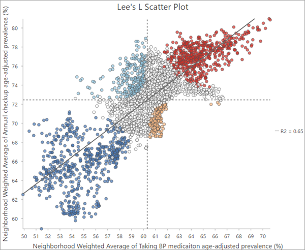
The output feature layer includes a Lee's L Scatter Plot chart that displays the neighborhood weighted averages of the first analysis variable on the x-axis and the neighborhood weighted averages of the second analysis variable on the y-axis, along with a linear trend line fit to the data. Dashed horizontal and vertical lines are also drawn at the mean value of each analysis variable. These lines divide the scatter plot into four quadrants and are used to divide the points into the local spatial association categories. For example, statistically significant features in the upper left quadrant will be the Low-High (light blue) category.

The chart can also be used to identify individual features that deviate from the general trends of the rest of the features. For example, you can select individual points in the scatter plot that fall far away from the trend line to further investigate these features. You may find that these features cluster together in the map and reveal regional patterns to the spatial associations that are otherwise difficult to detect.

Best practices and limitations

Consider the following when using this tool:

• Outliers (values that are much larger or smaller than the rest of the values) in either analysis variable will greatly affect the results. It is recommended that you create histograms of each analysis variable to determine whether outliers are present and to remove any features containing outliers in either variable. You can also use data engineering to identify outliers.
• When using this tool, it is assumed that there is a linear relationship between the neighborhood weighted averages of the two analysis variables. If the values in the Lee's L Scatter Plot chart display a pattern that is not linear, you can use the Transform Field tool to apply transformations to the analysis variables to linearize the relationship, and rerun the tool with the transformed values.
• A statistically significant p-value (generally less than 0.05) does not necessarily mean that there is cross correlation between the two variables. It could instead mean only that one or both of the variables have high spatial autocorrelation. To interpret a significant p-value, review the values of the global Lee's L statistic, the correlation between neighborhood averages, and the spatial smoothing scalar of each variable. Together, these values allow you to interpret the source of the statistical significance: autocorrelation, cross correlation, or both. If the p-value is significant, but global Lee's L statistic and correlation between neighborhood averages are very close to 0 and the spatial smoothing scalars are close to 1, it likely means that the variables are each highly autocorrelated, but there is little cross correlation between them.
• It is recommended that you use at least 50 input features and include at least 8 neighbors for each feature.

Formulas

This section contains the formulas for all statistics calculated by the tool. See the papers in the References section below for derivations and more information.

In all formulas, x refers to the first analysis variable, and y refers to the second analysis variable. A tilde (~) above a variable indicates that it is a weighted average of the neighborhood values. The weights for each neighborhood are normalized to sum to 1. A bar above a variable indicates that it is an unweighted average of all n input features. The subscript i indicates a single input feature. All sums in the formulas sum across all input features.

The global Lee's L statistic is calculated with the following formula:

The global Lee's L statistic is also approximately equal to the product of the square roots of the spatial smoothing scalars and the correlation between the neighborhood weighted averages as follows:

The spatial smoothing scalars are calculated with the following formulas:

The correlation between the neighborhood weighted averages is calculated with the following formula:

The local Lee's L statistics are calculated with the following formula:

The global Lee's L statistic is equal to the average of the local Lee's L statistics as follows:

References

The following resources were used to implement the tool:

• Lee, Sang-Il. "Developing a bivariate spatial association measure: an integration of Pearson's r and Moran's I." Journal of geographical systems 3 (2001): 369-385. https://doi.org/10.1007/s101090100064.
• Lee, Sang-Il. "A generalized randomization approach to local measures of spatial association." Geographical Analysis 41.2 (2009): 221-248. https://doi.org/10.1111/j.1538-4632.2009.00749.x.