How Forest-based Forecast works

The Forest-based Forecast tool uses forest-based regression to forecast future time slices of a space-time cube. The primary output is a map of the final forecasted time step as well as informative messages and pop-up charts. You can also create a new space-time cube containing the data from the original cube along with the forecasted values appended.

This tool uses the same underlying algorithm as the Forest-based Classification and Regression tool when used for regression. The training data used to build the forest regression model is constructed using time windows on each location of the space-time cube.

Learn more about Forest-based Classification and Regression

Potential applications

Forest regression models make few assumptions about the data, so they are used in many contexts. They are most effective compared to other forecasting methods when the data has complex trends or seasons, or changes in ways that do not resemble common mathematical functions such as polynomials, exponential curves, or sine waves.

For example, you can use this tool in the following applications:

• A school district can use this tool to forecast the number of students who will be absent on each day of the following week at each school in the district.
• Public utility managers can use this tool to forecast the electricity and water needs for next month in neighborhoods in their administrative district.
• Retail stores can use this tool to predict when individual products will be sold out in order to better manage inventory.

Forecasting and validation

The tool builds two models while forecasting each time series. The first is the forecast model, which is used to forecast the values of future time steps. The second is the validation model, which is used to validate the forecasted values.

Forecast model

The forecast model is constructed by building a forest with the time series values at each location of the space-time cube. This forest is then used to predict the next time slice. The forecasted value at the new time step is included into the forest model, and the next time step is forecasted. This recursive process continues for all future time steps. The fit of the forest to each time series is measured by the Forecast root mean square error (RMSE), which is equal to the square root of the average squared difference between the forest model and the values of the time series.

, where T is the number of time steps, c_t is the value of the forest model, and r_t is the raw value of the time series at time t.

The following image shows the raw values of a time series and a forest model fitted to the time series along with forecasts for two future time steps. The Forecast RMSE measures how much the fitted values from the forest differ from the raw time series values.

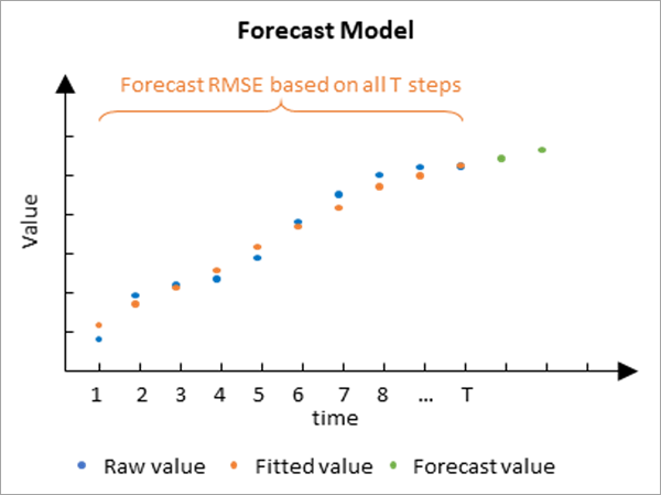
The Forecast RMSE only measures how well the forest model fits the raw time series values. It does not measure how well the forecast model actually forecasts future values. It is common for a forest model to fit a time series closely but not provide accurate forecasts when extrapolated. This problem is addressed by the validation model.

Validation model

The validation model is used to determine how well the forecast model can forecast future values of each time series. It is constructed by excluding some of the final time steps of each time series and fitting the forest model to the data that was not excluded. This forest model is then used to forecast the values of the data that were withheld, and the forecasted values are compared to the raw values that were hidden. By default, 10 percent of the time steps are withheld for validation, but this number can be changed using the Number of Time Steps to Exclude for Validation parameter. The number of time steps excluded cannot exceed 25 percent of the number of time steps, and no validation is performed if 0 is specified. The accuracy of the forecasts is measured by calculating a Validation RMSE statistic, which is equal to the square root of the average squared difference between the forecasted and raw values of the excluded time steps.

, where T is the number of time steps, m is the number of time steps withheld for validation, c_t is the value forecasted from the first T-m time steps, and r_t is the raw value of the time series withheld for validation at time t.

The following image shows a forest model fitted to the first half of a time series and then used to predict the second half of the time series. The Validation RMSE measures how much the forecasted values differ from the raw values at the withheld time steps.

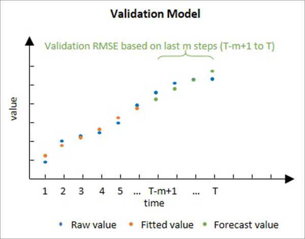
The validation model is important because it can directly compare forecasted values to raw values to measure how well the forest can forecast. While it is not actually used to forecast, it is used to justify the forecast model.

Note:

Validation in time series forecasting is similar but not identical to a common technique called cross validation. The difference is that forecasting validation always excludes the final time steps for validation, and cross validation either excludes a random subset of the data or excludes each value sequentially.

Interpretation

There are several considerations when interpreting the Forecast RMSE and Validation RMSE values.

• The RMSE values are not directly comparable to each other because they measure different things. The Forecast RMSE measures the fit of the forest model to the raw time series values, and the Validation RMSE measures how well the forest model can forecast future values. Because the Forecast RMSE uses more data and does not extrapolate, it is usually smaller than the Validation RMSE.
• Both RMSE values are in the units of the data. For example, if your data is temperature measurements in degrees Celsius, a Validation RMSE of 50 is very high because it means that the forecasted values differed from the true values by approximately 50 degrees on average. However, if your data is daily revenue in U.S. dollars of a large retail store, the same Validation RMSE of 50 is very small because it means that the forecasted daily revenue only differed from the true values by $50 per day on average.

Building and training the forest model

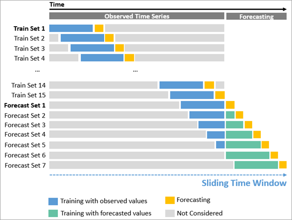
To forecast future values, the forest model must be trained by associating explanatory variables with dependent variables for each location. The forest model requires repeated training data, but there is only one time series for each location. To create multiple sets of explanatory and dependent variables within a single time series, time windows are constructed in which the time steps inside each time window are used as explanatory variables, and the next time step after the time window is the dependent variable. For example, if there are 20 time steps at a location, and the time window is 5 time steps, there are 15 sets of explanatory and dependent variables used to train the forest at that location. The first set has time steps 1, 2, 3, 4, and 5 as explanatory variables and time step 6 as the dependent variable. The second set has time steps 2, 3, 4, 5, and 6 as explanatory variables and time step 7 as the dependent variable. The final set has time steps 15, 16, 17, 18, and 19 as explanatory variables and time step 20 as the dependent variable. The number of time steps within each time window can be specified using the Time Step Window parameter. The time window can be as small as 1 (so that there is only a single time step within each time window) and cannot exceed one-third of the number of time steps at the location.

Using the trained forest model, the final time steps of the location are used as explanatory variables to forecast the first future time step. The second future time step is then forecasted using the previous time steps in the time window, where one of these time steps is the first forecasted value. The third forecasted time step similarly uses the previous time steps in the window, where two of these time steps are previous forecasted time steps. This process continues through all future time steps.

The following image shows the sets of explanatory and dependent variables used to train the forest model and forecast the first seven future time steps:

The forest forecast model is trained using time windows.

Seasonality and choosing a time window

The number of time steps within each time step window is an important choice for the forest model. A major consideration is whether the time series displays seasonality where natural cyclical patterns repeat over a certain number of time steps. For example, temperature displays yearly seasonal cycles according to seasons of the year. Because the time window is used to build associated explanatory and dependent variables, it is most effective when those explanatory variables all come from the same seasonal cycle so that there is as little seasonal correlation between the explanatory variables as possible. It is recommended that you use the number of time steps in a natural season for the length of the time step window. If your data displays multiple seasons, it is recommended that you use the length of the longest season.

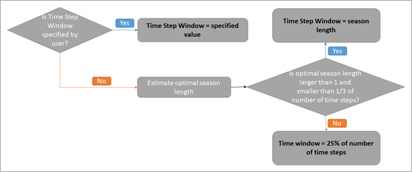
If you know the number of time steps that correspond to one season in your data, you can specify it in the Time Step Window parameter, and this value will be used by every location in the space-time cube. If you do not know the length of a season or if the seasonal length is different for different locations, the parameter value can be left empty, and an optimal season length will be estimated for each location using a spectral density function. For details about this function, see the Additional resources section.

For an individual location, if the optimal season length determined by spectral analysis is greater than one and not greater than one-third of the number of time steps at the location, the time step window is set to this optimal value. Otherwise, the location uses 25 percent (rounded down) of the number of time steps at the location for the time step window. This ensures that there is at least one time step in the window and that at least three full seasonal cycles are used as explanatory variables. The time step value used at the location is saved in the Time Window field of the output features. The Is Seasonal field of the output features will contain the value 1 if the time step window was determined using spectral analysis and will contain 0 otherwise. This workflow is summarized in the following image:

The time step window can be specified or estimated for each location by detecting seasonality.

Approaches to forecasting

There are four ways you can represent the values of the explanatory and dependent variables that will be used to train the forest. These options are specified using the Forecast Approach parameter.

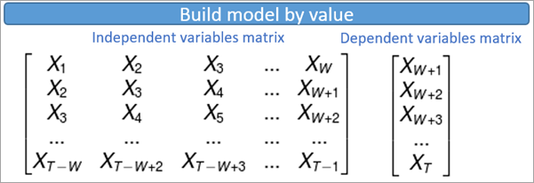
The first option is Build model by value. This option uses the raw values in the space-time bins for the explanatory and dependent variables. When this option is chosen, the forecasted values will be contained within the range of the dependent variables, so you should not use this option if your data has trends where you expect the values to continue to increase or decrease when forecasting the future. The image below shows the sets of variables used to train the model for a single location in which each row displays the set of explanatory variables and the associated dependent variable. T is the number of time steps in the space-time cube, W is the number of time steps in each time step window, and X_t is the raw value of the time series at time t.

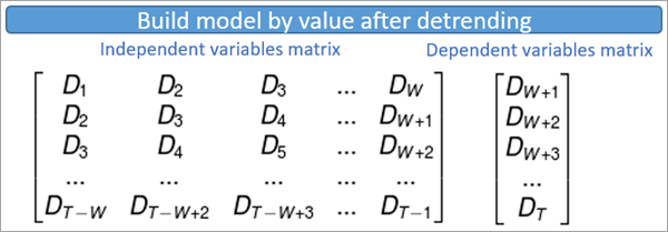
The second option is Build model by value after detrending. This is the default option of the tool. This option performs a first-order (linear) trend removal on the entire time series at each location, and these detrended values are used as the explanatory and dependent variables. Using this option allows the forecasts to follow this trend into the future so that the forecasted values can be estimated outside of the range of the dependent variables. The image below shows the sets of variables used to train the model for a single location in which each row displays the set of explanatory variables and the associated dependent variable. T is the number of time steps in the space-time cube, W is the number of time steps in each time step window, and D_t is the detrended value of the time series at time t.

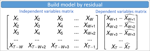
The third option is Build model by residual. This option creates an ordinary least-squares (OLS) regression model to predict the dependent variable based on the explanatory variables within each time window. The residual of this regression model (the difference between the OLS prediction and the raw value of the dependent variable) is used to represent the dependent variable when training the forest. The image below shows the sets of variables used to train the model for a single location in which each row displays the set of explanatory variables and the associated dependent variable. T is the number of time steps in the space-time cube, W is the number of time steps in each time step window, X_t is the value of the time series at time t, and X^{^}_t (X_t-hat) is the value estimated from OLS at time t.

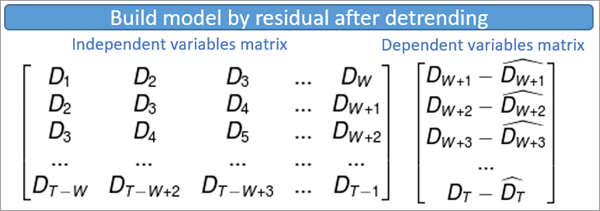
The last option is Build model by residual after detrending. This option first performs a first-order (linear) trend removal on the entire time series at a location. It then builds an OLS regression model to predict the detrended dependent variable based on the detrended explanatory variables within each time window. The residual of this regression model (the difference between the OLS prediction and the detrended value of the dependent variable) is used to represent the dependent variable when training the forest. The image below shows the sets of variables used to train the model for a single location in which each row displays the set of explanatory variables and the associated dependent variable. T is the number of time steps in the space-time cube, W is the number of time steps in each time step window, D_t is the detrended value of the time series at time t, and D^{^}_t (D_t-hat) is the value estimated from OLS at time t.

Constructing confidence intervals

The tool calculates 90 percent confidence intervals for each forecasted time step that appear as fields in the Output Features and display in the pop-up charts discussed in the next section. The upper and lower bounds of the confidence interval for the first forecasted time step are calculated using quantile random forest regression. To predict the value of a future time, the observations within each leaf of a tree are averaged together. In quantile regression, however, each observation within each leaf is used, and this results in a distribution of forecasted values for the first time step. The 90 percent confidence interval is constructed using the 5th and 95th quantiles of this distribution.

The confidence interval for the second forecast is computed in a similar way but is adjusted taking into account the confidence interval of the first forecast. Quantile regression is again used to create a distribution for the second forecasted time step, treating the first forecasted time step as a singular value, and the 5th and 95th quantiles of the distribution are calculated. The actual confidence for the second forecast is calculated by adding the lengths of the confidence bounds of both forecasts. The upper bound of the second forecast is equal to the length of the upper bound for the first forecast plus the length of the upper confidence bound for the second forecast (calculated assuming the first forecast is a single value instead of a distribution). The lower bound is similarly calculated by adding the lengths of the lower confidence bounds. The confidence interval for the third forecasted time step is computed by performing quantile regression again and adding the lengths of the error bounds for all three forecasts. This process continues until all time steps are forecasted. Adding these error bounds in this way ensures that the error is propagated forward through the projections and that the lengths of the confidence bands increase going forward in time.

Note:

The confidence bounds for the second time step and beyond are calculated conservatively by adding errors of previous forecasts. The actual confidence level of these intervals is at least 90 percent, but they could actually be at a higher confidence level.

Tool outputs

The primary output of this tool is a 2D feature class showing each location in the Input Space Time Cube symbolized by the final forecasted time step with the forecasts for all other time steps stored as fields. Although each location is independently forecasted and spatial relationships are not taken into account, the map may display spatial patterns for areas with similar time series.

Pop-up charts

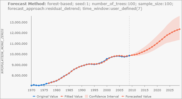
Clicking any feature on the map using the Explore navigation tool displays a chart in the Pop-up pane showing the values of the space-time cube along with the fitted forest model and the forecasted values along with 90 percent confidence intervals for each forecast. The values of the space-time cube are displayed in blue and are connected by a blue line. The fitted values are displayed in orange and are connected by a dashed orange line. The forecasted values are displayed in orange and are connected by a solid orange line representing the forecasting of the forest model. Light red confidence bounds are drawn around each forecasted value. You can hover over any point in the chart to see the date and value of the point.

The pop-up chart displays the original values, fitted values, forecasted values, and confidence intervals.

Note:

Pop-up charts are not created when the output features are saved as a shapefile (.shp). Additionally, if the confidence intervals extend off the chart, a Show Full Data Range button appears above the chart that allows you to extend the chart to show the entire confidence interval.

Geoprocessing messages

The tool provides a number of messages with information about the tool execution. The messages have three main sections.

The Input Space Time Cube Details section displays properties of the input space-time cube along with information about the number of time steps, number of locations, and number of space-time bins. The properties displayed in this first section depend on how the cube was originally created, so the information varies from cube to cube.

The Analysis Details section displays properties of the forecast results, including the number of forecasted time steps, the number of time steps excluded for validation, the percent of locations where seasonality was detected by spectral analysis, and information about the forecasted time steps. If a value is not provided for the Time Step Window parameter, summary statistics of the estimated time step window are displayed, including the minimum, maximum, average, median, and standard deviation.

The Summary of Accuracy across Locations section displays summary statistics for the Forecast RMSE and Validation RMSE among all of the locations. For each value, the minimum, maximum, mean, median, and standard deviation is displayed.

Note:

Geoprocessing messages appear at the bottom of the Geoprocessing pane during tool execution. You can access the messages by hovering over the progress bar, clicking the pop-out button , or expanding the messages section in the Geoprocessing pane. You can also access the messages for a previously run tool using geoprocessing history.

Fields of the output features

In addition to Object ID, geometry fields, and the field containing the pop-up charts, the Output Features will have the following fields:

• Location ID (LOCATION)—The Location ID of the corresponding location of the space-time cube.
• Forecast for (Analysis Variable) in (Time Step) (FCAST_1, FCAST_2, and so on)—The forecasted value of each future time step. The field alias displays the name of the Analysis Variable and the date of the forecast. A field of this type is created for each forecasted time step.
• High Interval for (Analysis Variable) in (Time Step) (HIGH_1, HIGH_2, and so on)—The upper bound of a 90 percent confidence interval for the forecasted value of each future time step. The field alias displays the name of the Analysis Variable and the date of the forecast. A field of this type is created for each forecasted time step.
• Low Interval for (Analysis Variable) in (Time Step) (LOW_1, LOW_2, and so on)—The lower bound of a 90 percent confidence interval for the forecasted value of each future time step. The field alias displays the name of the Analysis Variable and the date of the forecast. A field of this type is created for each forecasted time step.
• Forecast Root Mean Square Error (F_RMSE)—The Forecast RMSE.
• Validation Root Mean Square Error (V_RMSE)—The Validation RMSE. If no time steps were excluded for validation, this field is not created.
• Time Window (TIMEWINDOW)—The time step window used at the location.
• Is Seasonal (IS_SEASON)—A Boolean variable indicating whether the time step window at the location was determined by spectral density. A value of 1 indicates seasonality was detected by spectral density, and a value of 0 indicates no seasonality was detected. If a value is specified in the Time Window parameter, all locations have the value 0 in this field.
• Forecast Method (METHOD)—A text field displaying the parameters of the forest model, including the random seed, number of trees, sample size, forecast approach, and whether the time step window was specified by the user or determined by the tool. This field can be used to reproduce results, and it allows you to identify which models are used in the Evaluate Forecasts By Location tool.

Output space-time cube

If an Output Space Time Cube is specified, the output cube contains all of the original values from the input space-time cube with the forecasted values appended. This new space-time cube can be displayed using the Visualize Space Time Cube in 2D or Visualize Space time Cube in 3D tools and can be used as input to the tools in the Space Time Pattern Mining toolbox, such as Emerging Hot Spot Analysis and Time Series Clustering.

Multiple forecasted space-time cubes can be compared and merged using the Evaluate Forecasts by Location tool. This allows you to create multiple forecast cubes using different forecasting tools and parameters, and the tool identifies the best forecast for each location using either Forecast or Validation RMSE.

Best practices and limitations

When deciding whether this tool is appropriate for your data and which parameters you should choose, several things should be taken into account.

• Compared to other forecasting tools in the Time Series Forecasting toolset, this tool is the most complicated but makes the fewest assumptions about the data. It is recommended for time series with complicated shapes and trends that are difficult to model with simple or smooth mathematical functions. It is also recommended when the assumptions of other methods are not satisfied.
• Deciding how many time steps to exclude for validation is important. The more time steps are excluded, the fewer time steps remain to estimate the validation model. However, if too few time steps are excluded, the Validation RMSE is estimated using a small amount of data and may be misleading. It is recommended that you exclude as many time steps as possible while still maintaining sufficient time steps to estimate the validation model. It is also recommended that you withhold at least as many time steps for validation as the number of time steps you intend to forecast, if your space-time cube has enough time steps to allow this.
• This tool may produce unstable and unreliable forecasts when the same value is repeated many times within the time series. A common source of repeated identical values is zero-inflation, in which your data represents counts and many of the time steps have the value 0.

Additional resources

For more information about forest models, see the following references:

• Breiman, Leo. (2001). "Random Forests." Machine Learning 45 (1): 5-32. https://doi.org/10.1023/A:1010933404324.
• Breiman, L., J.H. Friedman, R.A. Olshen, and C.J. Stone. (2017). Classification and regression trees. New York: Routledge. Chapter 4.

For additional resources and references for forest models, see How Forest-based Classification and Regression works.

For more information about the spectral density function used to estimate the length of time windows, see the findfrequency function in the following references:

• Hyndman R, Athanasopoulos G, Bergmeir C, Caceres G, Chhay L, O'Hara-Wild M, Petropoulos F, Razbash S, Wang E, and Yasmeen F (2019). "Forecasting functions for time series and linear models." R package version 8.7, https://pkg.robjhyndman.com/forecast.
• Hyndman RJ and Khandakar Y (2008). "Automatic time series forecasting: the forecast package for R." Journal of Statistical Software, 26(3), pp. 1-22. https://www.jstatsoft.org/article/view/v027i03.

For more information about constructing confidence intervals from forest regression models, see the following reference:

• Meinshausen, Nicolai. "Quantile regression forests." Journal of Machine Learning Research 7. Jun (2006): 983-999.