For each location in a space-time cube, the Change Point Detection tool identifies time steps when some statistical property of the time series changes. The tool can detect changes in the mean value or standard deviation of continuous variables, as well as changes in the mean of count variables. The number of change points at each location can be determined by the tool or a defined number of change points can be provided that is used for all locations.
The change points divide each time series into segments, where the values within each segment have a similar mean or standard deviation. Change points are defined as the first time step in each new segment, so the number of change points is always one less than the number of segments.
Types of change points
Three types of change can be detected by the tool. Each image below shows the time series as a blue line chart with vertical orange lines at the change points.
- Mean shift—Detects shifts in the mean value of the analysis variable. The data values are assumed to follow a normal distribution with all time steps having the same standard deviation. The mean value is constant within each segment and changes to a new value at each change point.
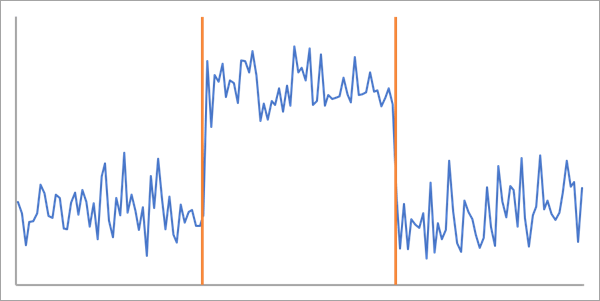
- Potential application—Detect heat waves when the daily maximum temperature increases over a short time span.
- Standard deviation—Detects changes in the standard deviation of the analysis variable. The data values are assumed to follow a normal distribution with all time steps having the same mean value. The standard deviation is constant within each segment and changes to a new value at each change point.
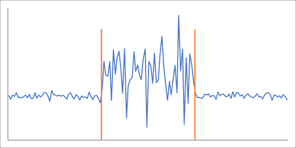
- Potential application—Detect changes in the variation of wind velocity that could indicate major weather events.
- Count—Detects changes in the mean value of an analysis variable representing counts. The data values are assumed to follow a Poisson distribution within each
segment with a mean that changes to a new value at each change point.
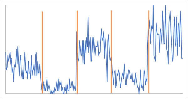
- Potential application—Detect changes in daily influenza counts to estimate the beginning and end of each annual flu season.
Tool outputs
The primary output of the tool is a feature class with one feature for each location of the input space-time cube. The layer is drawn with five classes based on the number of change points detected at each location.
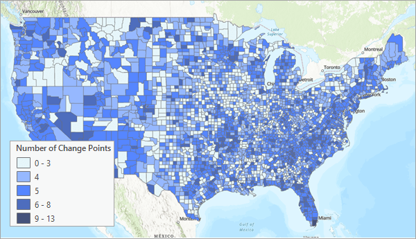
The output features include the following fields:
- Number of Change Points (NUM_CPTS)—The number of change points detected at the location.
- Date of First Change Point (FIRST_CHPT)—The date of the first change point at the location. If no change points are detected, the value will be null.
- Date of Last Change Point (LAST_CHPT)—The date of the last change point at the location. If no change points are detected, the value will be null. If one change point is detected, the value will be the same as the date of the first change point.
The layer time of the output features is based on the date of the first change point, so the time slider can be used to filter locations based on this date. The layer time can be changed to the date of the last change point in the layer properties. This can be used, for example, to animate through time to visualize when different locations experience their first or last change point to identify temporal patterns across locations.
Time series pop-up charts
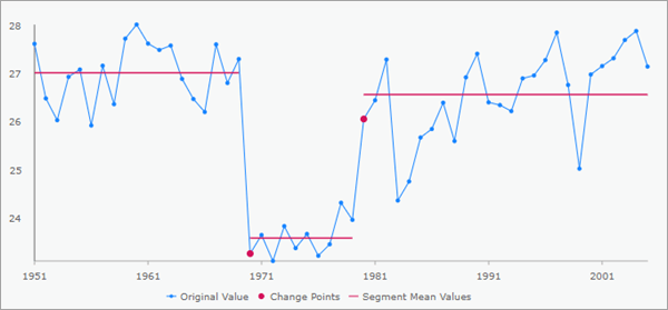
Clicking any feature on the map using the Explore navigation tool displays a line chart in the Pop-up pane. The chart displays a blue line chart of the time series at the location with change points indicated by larger red dots.
For the Mean shift and Count change types, horizontal red lines are drawn at the mean value of each segment.
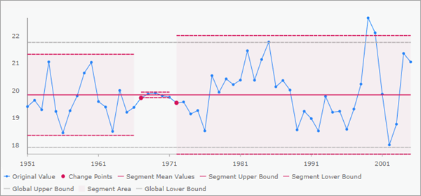
For the Standard deviation change type, a solid red line is drawn at the global mean value of the entire time series. For each segment, dashed red lines are drawn two standard deviations above and below the global mean with pink shading between the bands. These bands widen or narrow when the standard deviation changes at the change points. Dashed gray lines are drawn two global standard deviations above and below the global mean. This allows you to determine whether the standard deviation of a segment is larger or smaller than the standard deviation of the entire time series.
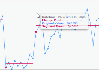
You can hover over any element in the chart to get more information about the values.
Note:
Pop-up charts are not created when the output features are saved as a shapefile (.shp).
Geoprocessing messages
The tool provides a number of messages with information about the tool execution. The messages have several sections.
The Input Space Time Cube Details section displays properties of the input space-time cube along with information about the time step interval, number of time steps, number of locations, and number of space-time bins. The properties displayed in this first section depend on how the cube was created, so the information varies from cube to cube.
The Important Dates section displays the dates of the first and last change point across all locations as well as the date with the most change points. This can be used to identify dates when large changes occurred that caused changes in multiple locations. If there are ties, the earliest date is displayed.
The Summary of Number of Change Points Per Time Step section displays the minimum, maximum, mean, median, and standard deviation for the number of change points per time step. This allows you to investigate the frequency of change points across the time series across all locations. If the frequency is too high or too low, you can adjust the value of the Detection Sensitivity parameter to increase or decrease the frequency of change points.
Visualize the space-time cube in 3D
The input space-time cube is updated with the results of the analysis and can be used in the Visualize Space Time Cube in 3D tool with the Time series change points option of the Display Theme parameter to display the results in a 3D scene. The output will contain one feature per time step of the space-time cube. Time steps detected as change points are labeled Change Point and display in purple, and time steps not detected as change points are labeled Not a Change Point and display in light gray.
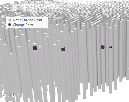
Informational fields about the time, location, and ID of the time step are included along with the following fields about the detected change points:
- Change Point Indicator (CHPT_IND)—The field contains the value 1 if the time step is detected as a change point and contains 0 if the time step is not detected as a change point.
- Current Mean (MEAN_CUR)—The mean value of the segment containing the time step. This field is only created for the mean shift change type.
- Mean Before (MEAN_BEF)—The mean value of the segment containing the previous time step. The Current Mean and Mean Before values will be equal if the time step is not a change point and will be different if the time step is a change point (because the previous value is in a different segment). This allows you to compare the mean values of the segments before and after the change point. This field is only created for the mean shift change type.
- Current Standard Deviation (STDEV_CUR)—The standard deviation of the segment containing the time step. This field is only created for the standard deviation change type.
- Standard Deviation Before (STDEV_BEF)—The standard deviation of the segment containing the previous time step. The Current Standard Deviation and Standard Deviation Before values will be equal if the time step is not a change point and will be different if the time step is a change point. This field is only created for the standard deviation change type.
- Current Mean of Counts (MEAN_CUR)—The mean value of the counts of the segment containing the time step. This field is only created for the count change type.
- Mean of Counts Before (MEAN_BEF)—The mean value of the counts of the segment containing the previous time step. The Current Mean of Counts and Mean of Counts Before values will be equal if the time step is not a change point and will be different if the time step is a change point. This field is only created for the count change type.
Note:
The Time series change points display theme of the Visualize Space Time Cube in 2D tool will re-create the required output feature class of change point detection.
How change points are detected
The goal of change point detection is to find time steps when the mean or standard deviation of the data changes from one value to another. This problem is equivalent to the problem of time series segmentation, where a time series is divided into segments whose values each have a similar mean or standard deviation. To determine which segmentation (set of change points) is optimal for a time series, you must be able to measure and compare the effectiveness of different possible segmentations. This comparison is performed by calculating a segmentation cost for each segmentation, and the one with the lowest cost is most optimal.
The cost of a segmentation is calculated by adding the individual costs of each segment in the segmentation, where the cost of each segment is based on a likelihood function determined by the change type (see Types of change points for the distributional assumptions of each change type). Intuitively, the closer the segments follow the assumed distribution of the change type, the higher the likelihood and the lower the cost of the segmentation.

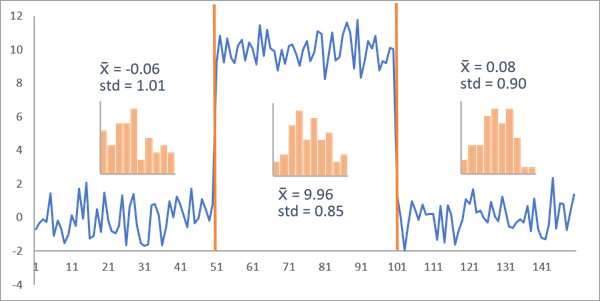
For example, the image below shows a time series with 150 time steps where all values were generated from a normal distribution with standard deviation equal to 1. The mean of the first 50 time steps is 0, then the mean increases to 10 for the middle 50 time steps, then decreases back to 0 for the final 50 time steps. Change points are defined as the first time steps in each new segment, so for this time series, time steps 51 and 101 are the true change points when the mean shifts. The histograms of the individual segments show that each segment appears to follow a normal distribution with approximately equal standard deviation but different mean value, so this segmentation appears to align with the assumptions of the mean shift change type. This indicates that the likelihood of this segmentation is high, and the resulting segmentation cost is low. For this correct segmentation, the segmentation cost is 401.39 when detecting mean shift. This value is difficult to interpret on its own, but it can be compared to the cost of other possible segmentations.
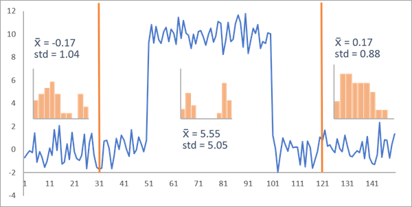
The image below shows an incorrect segmentation where time steps 31 and 121 are detected as change points. The middle segment does not appear normally distributed and has a much larger standard deviation than the first and last segments. This suggests that the data values of the segments are unlikely under the distributional assumption of the mean shift change type, so the segmentation cost should be high. Indeed, the cost of this segmentation is 2596.24, which is much larger than the cost of the correct segmentation. This confirms that these change points are not optimal for this time series.
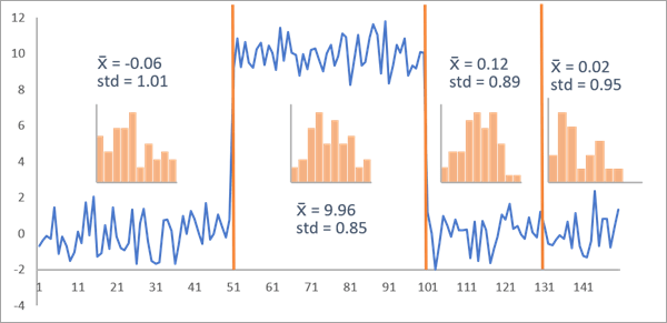
Now, suppose an unnecessary change point is added in addition to the two true change points. In the image below, time steps 51, 101, and 131 are identified as change points. While the last change point is unnecessary, the segment histograms do appear normally distributed with approximately equal standard deviation, indicating a high likelihood and low segmentation cost. The cost of this segmentation is 401.27, which is slightly lower than the cost of the true segmentation (401.39). The segmentation with an unneeded change point has a lower segmentation cost than the true segmentation because likelihoods never decrease by including new parameters (in this case, new change points). The inclusion of the extra change point only decreased the cost by a small amount because it provided very little improvement to the fit of the model to the data, compared to not being included as a change point.
If no constraints are applied on the number of change points, the segmentation cost will always decrease by adding more change points. To prevent all time steps from being detected as change points, you must apply one of two types of constraints using the Method parameter.
The Defined number of change points (SegNeigh) option allows you to specify how many change points to detect using the Number of Change Points parameter. This option uses the Segment Neighborhood (SegNeigh, Auger 1989) algorithm to find the segmentation with the lowest cost among all possible segmentations that have the specified number of change points.
The Auto-detect number of change points (PELT) option uses the Pruned Exact Linear Time (PELT, Killick 2012) algorithm to estimate the number and location of change points. This algorithm penalizes the inclusion of each additional change point by adding a penalty value to the cost of each segment and finding the segmentation whose penalized cost (segmentation cost plus penalty) is smallest among all possible segmentations. The intuition behind PELT is that for a time step to be detected as a change point, it must reduce the segmentation cost by more than the penalty value that is added. If the cost reduction is less than the added penalty, the penalized cost will increase, and the time step will not be detected as a change point.
The choice of the penalty value is critical to the results of PELT. Penalties that are too low can detect many false change points, and penalties that are too high can fail to detect true change points. The penalty value used in PELT is determined by the value of the Detection Sensitivity parameter. The sensitivity is provided as a number between 0 and 1, where higher sensitivities detect more change points by using lower penalty values. The penalty value is determined from the sensitivity using the following formula, where n is the number of time steps in the time series:

The highest sensitivity value of 1 corresponds to minimizing the Bayesian Information Criterion (BIC). Because the penalty value only depends on the number of time steps, all locations of the space-time cube will use the same penalty value.
PELT and SegNeigh are both exact recursive algorithms, meaning that they will always return the segmentation with the globally smallest segmentation cost, given a fixed penalty value or fixed number of change points. The algorithms are performed independently on all locations of the input space-time cube.
There is a correspondence between PELT and SegNeigh in that they will detect the same time steps as change points if both methods detect the same number of change points. For example, if you perform PELT and use a penalty value that detects six change points at a location, then perform SegNeigh and specify six change points to be detected, both methods will detect the same time steps as change points.
Best practices and limitations
Several considerations should be made when choosing the parameters and options of the tool.
- Change point detection methods are classified as being online or offline, and this tool performs offline detection. Offline methods assume an existing time series with a start and end, and the goal is to look back in time to determine when changes occurred. Online methods instead constantly run on data that is updated as new values become available. The goal of online detection methods is live detection of new changes in as little time as possible after the change has occurred. Online and offline methods differ significantly in their algorithms, use cases, and assumptions about the data.
- This tool is most effective for data without trends and whose changes occur in a single time step. For time series with trends, many time steps may be detected as change points due to the constantly changing mean value. Similarly, if the change is more gradual and takes several time steps before the value fully changes, all time steps during the transition may be detected as change points. For these cases, it is recommended that you use lower values for the Detection Sensitivity parameter.
- Change point detection is similar to time series outlier detection but differs in important ways. Change point detection identifies time steps when one model changes to a new model (such as a change in the mean value), and outlier detection identifies time steps that deviate significantly from a single model. The former suggests a sustained change while the latter suggests a short-term anomaly.
For analysis variables that represent counts, the Count option of the Change Type parameter is often most appropriate for detecting changes in the mean value of the counts. However, the Mean shift option may provide equivalent or better results for count data. This is because the model of the count change type assumes that the values of each segment follow a Poisson distribution in which the variance of the segment is equal to the mean value of the segment. The mean shift change type instead assumes that the values of each segment are normally distributed, so the mean value can be larger or smaller than the variance of the values.
In a Poisson distribution, most counts are within approximately two square roots of the mean value. For example, for a Poisson distribution with a mean value equal to 100, approximately 95 percent of the counts will be between 80 and 120 (2 * sqrt(100) = 20). For a Poisson distribution with a mean equal to 1 million, most counts will be between 998,000 and 1,002,000 (the square root of 1 million is 1,000). The range of counts is comparatively more narrow for the larger mean of 1 million, where most counts are within 0.2 percent of the mean value. In the smaller mean of 100, however, counts vary up to 20 percent from the mean value. Compared to their mean value, if the values of your counts vary more than expected from a Poisson distribution, many time steps may be detected as change points. This is most common with large counts. In this case, it is recommended that you detect mean shift.
- For all change types, the first time step will never be detected as a change point. This is because change points mark the beginning of each new segment, starting with the second segment. Because the first time step is always in the first segment, it can never be a change point.
- For the Defined number of change points (SegNeigh) option of the Method parameter, the optimal segmentation is not always unique. If multiple segmentations have the same segmentation cost, the latest possible optimal change points will be returned. For example, if all values of a time series are equal at a location, all segmentations have the same likelihood and cost. In this case, if three change points are requested, the final three time steps will be detected as change points at the location.
- Detecting mean shift requires estimating the variance of the data around the mean without already knowing the time steps where the mean shifts (the change points). Traditional variance formulas are biased in the presence of an unknown changing mean, so the following robust variance formula is used:

If this formula evaluates to zero, the variance is estimated assuming no shifts in the mean value.
Additional resources
For more information about change point detection, see the following references:
- Auger, I. E. and Lawrence, C. E. (1989). "Algorithms for the optimal identification of segment neighborhoods." Bulletin of Mathematical Biology. 51(1):39-54. https://doi.org/10.1007/BF02458835
- Killick, R., Fearnhead, P., and Eckley, I.A. (2012). "Optimal Detection of Changepoints With a Linear Computational Cost." Journal of the American Statistical Association. 107. 1590-1598. https://dx.doi.org/10.1080/01621459.2012.737745
- Killick, R. and Eckley, I.A. (2014). "changepoint: An R Package for Changepoint Analysis." Journal of Statistical Software. https://dx.doi.org/10.18637/jss.v058.i03