How Forest-based Forecast works

The Forest-based Forecast tool uses forest-based regression to forecast future time slices of a space-time cube. The primary output is a map of the final forecasted time step as well as informative messages and pop-up charts. Other explanatory variables can be provided to improve the forecast of the analysis variable, and you can estimate and visualize lagged effects between the explanatory variables and the variable being forecasted. You can also choose to build forest-based models on each location independently, build a single model trained from all locations, or build separate models within each time series cluster. Additionally, you have the option to detect outliers in each time series to identify locations and times that significantly deviate from the patterns and trends of the rest of the time series.

This tool uses the same underlying algorithm as the Forest-based Classification and Regression tool when used for regression. The training data used to build the forest regression model is constructed using time windows on each variable of the space-time cube.

Learn more about Forest-based Classification and Regression

Potential applications

Forest regression models make few assumptions about the data, so they are used in many contexts. They are most effective compared to other forecasting methods when the data has complex trends or seasons, or changes in ways that do not resemble common mathematical functions such as polynomials, exponential curves, or sine waves.

For example, you can use this tool in the following applications:

• A school district can use this tool to forecast the number of students who will be absent on each day of the following week at each school in the district.
• A governor can predict the number of hospitalizations from an infectious disease two weeks in the future. This forecast can include the number of positive test results as an explanatory variable, and the tool will model the delayed effect between positive tests and hospitalizations.
• Public utility managers can use this tool to forecast the electricity and water needs for next month in neighborhoods in their administrative district.
• Retail stores can use this tool to predict when individual products will be sold out in order to better manage inventory.
• City planners can use this tool to predict future populations to assess demand for housing, energy, food, and infrastructure. Cities with similar sizes and population trends can be grouped together in a cluster, and forest-based models can be built for each group.

Forecasting and validation

The tool builds two models while forecasting each time series. The first is the forecast model, which is used to forecast the values of future time steps. The second is the validation model, which is used to validate the forecasted values.

Note:

This section describes the Individual location option of the Model Scale parameter. The Entire cube and Time series cluster options operate analogously. See Extending model scale for more information.

Forecast model

The forecast model is constructed by building a forest with the time series values at each location of the space-time cube. This forest is then used to predict the next time slice. The forecasted value at the new time step is included into the forest model, and the next time step is forecasted. This recursive process continues for all future time steps. The fit of the forest to each time series is measured by the Forecast root mean square error (RMSE), which is equal to the square root of the average squared difference between the forest model and the values of the time series.

, where T is the number of time steps, c_t is the value of the forest model, and r_t is the raw value of the time series at time t.

The following image shows the raw values of a time series and a forest model fitted to the time series along with forecasts for two future time steps. The Forecast RMSE measures how much the fitted values from the forest differ from the raw time series values.

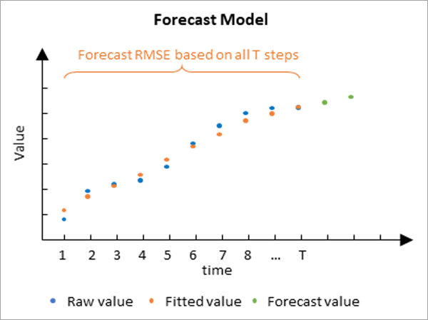
The Forecast RMSE only measures how well the forest model fits the raw time series values. It does not measure how well the forecast model actually forecasts future values. It is common for a forest model to fit a time series closely but not provide accurate forecasts when extrapolated. This problem is addressed by the validation model.

Validation model

The validation model is used to determine how well the forecast model can forecast future values of each time series. It is constructed by excluding some of the final time steps of each time series and fitting the forest model to the data that was not excluded. This forest model is then used to forecast the values of the data that were withheld, and the forecasted values are compared to the raw values that were hidden. By default, 10 percent of the time steps are withheld for validation, but this number can be changed using the Number of Time Steps to Exclude for Validation parameter. The number of time steps excluded cannot exceed 25 percent of the number of time steps, and no validation is performed if 0 is specified. The accuracy of the forecasts is measured by calculating a Validation RMSE statistic, which is equal to the square root of the average squared difference between the forecasted and raw values of the excluded time steps.

, where T is the number of time steps, m is the number of time steps withheld for validation, c_t is the value forecasted from the first T-m time steps, and r_t is the raw value of the time series withheld for validation at time t.

The following image shows a forest model fitted to the first half of a time series and used to predict the second half of the time series. The Validation RMSE measures how much the forecasted values differ from the raw values at the withheld time steps.

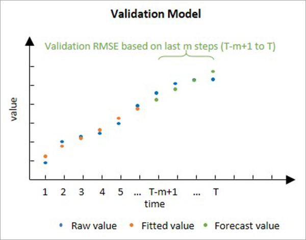
The validation model is important because it can directly compare forecasted values to raw values to measure how well the forest can forecast. While it is not actually used to forecast, it is used to justify the forecast model.

Note:

Validation in time series forecasting is similar but not identical to a common technique called cross validation. The difference is that forecasting validation always excludes the final time steps for validation, and cross validation either excludes a random subset of the data or excludes each value sequentially.

Interpretation

There are several considerations when interpreting the Forecast RMSE and Validation RMSE values.

• The RMSE values are not directly comparable to each other because they measure different things. The Forecast RMSE measures the fit of the forest model to the raw time series values, and the Validation RMSE measures how well the forest model can forecast future values. Because the Forecast RMSE uses more data and does not extrapolate, it is usually smaller than the Validation RMSE.
• Both RMSE values are in the units of the data. For example, if your data is temperature measurements in degrees Celsius, a Validation RMSE of 50 is very high because it means that the forecasted values differed from the true values by approximately 50 degrees on average. However, if your data is daily revenue in U.S. dollars of a large retail store, the same Validation RMSE of 50 is very small because it means that the forecasted daily revenue only differed from the true values by $50 per day on average.

Build and train the forest model

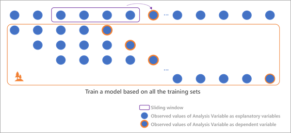
To forecast future values, the forest model must be trained by associating explanatory variables with dependent variables for each location. The forest model requires repeated training data, but there is only one time series for each location. To create multiple sets of explanatory and dependent variables within a single time series, time windows are constructed in which the time steps inside each time window are used as explanatory variables, and the next time step after the time window is the dependent variable. For example, if there are 20 time steps at a location, and the time window is 4 time steps, there are 16 sets of explanatory and dependent variables used to train the forest at that location. The first set has time steps 1, 2, 3, and 4 as explanatory variables and time step 5 as the dependent variable. The second set has time steps 2, 3, 4, and 5 as explanatory variables and time step 6 as the dependent variable. The final set has time steps 16, 17, 18, and 19 as explanatory variables and time step 20 as the dependent variable. The number of time steps within each time window can be specified using the Time Step Window parameter. The time window can be as small as 1 (so that there is only a single time step within each time window) and cannot exceed one-third of the number of time steps at the location.

The forest forecast model is trained using time windows.

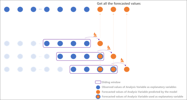
Using the trained forest model, the final time steps of the location are used as explanatory variables to forecast the first future time step. The second future time step is then forecasted using the previous time steps in the time window, where one of these time steps is the first forecasted value. The third forecasted time step similarly uses the previous time steps in the window, where two of these time steps are previous forecasted time steps. This process continues through all future time steps.

The following image shows the sets of explanatory and dependent variables used to train the forest model and forecast the first seven future time steps:

Forecasts are created using time windows.

Extend model scale

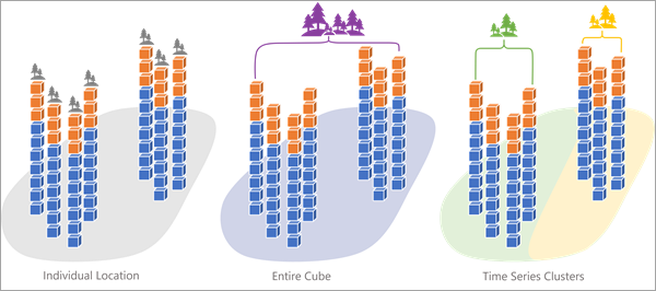
In addition to building separate forecast models at each location, you can group locations together and build a single forecast model that is used by all locations in the group. Grouping locations allows you to perform analysis at different scales, for example, models of city populations grouped by the overall population size. You can also build a global model with all locations in the same group.

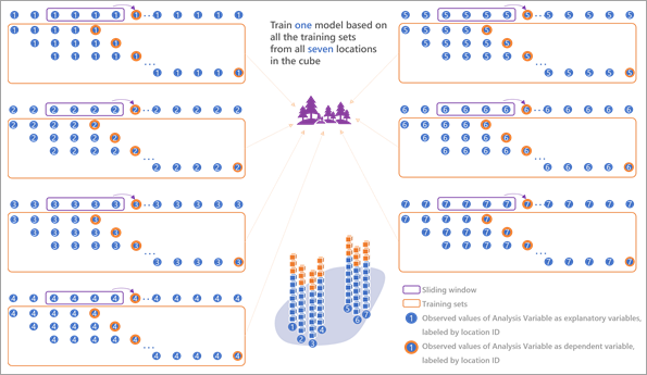
When grouped together, the shared forecast model uses the time windows of every location in the group as training data, so it has much more data from which to learn the patterns and trends of the time series than any individual location. This is especially important for short time series where there is limited training data available within each time series. When all the time series in the group have similar values and patterns, this extra training data allows more accurate forecasts of every location in the group by incorporating the patterns of the other locations. However, if the time series of the locations in the group have significantly different values and patterns, incorporating their patterns will reduce the accuracy of the forecasts, so it is important to only group time series that are similar.

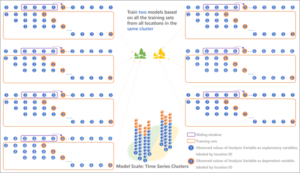
You can define the scale of analysis with the Model Scale parameter. The default Individual location option builds independent models at every location for a local-scale analysis. The Entire cube option builds a single model using all locations for a global-scale analysis. The Time series cluster option builds a model for each cluster of a time series clustering result for an analysis at the scale of the clusters (if the clusters form regions, it is a regional-scale analysis). The variable containing time series clustering results is provided in the Cluster variable parameter.

Three model scales can be used to build the forecast models.

The following image shows an example of building a single model for the entire cube with seven locations:

A single model is built using all locations as training data.

The following image shows an example of building separate models for each of two time series clusters:

A different model is built for each time series cluster.

Include other variables and the lag effect

While forest regression models can effectively capture complex patterns and trends of the time series, you can improve them by including additional information from other related variables. For example, knowing pollution levels can help forecast the number of emergency room visits due to asthma because pollution is a known trigger for asthma attacks.

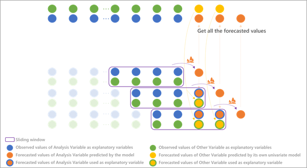
You can include related variables stored in the same space-time cube using the Other Variables parameter to forecast the analysis variable using a multivariate forest-based forecast. To train the multivariate forest regression model, each other variable is included within each time window and used to predict the next value after the time window, analogous to how time windows are used for the analysis variable, as described in the Build and train the forest model section.

The forest forecast model is trained using multiple variables.

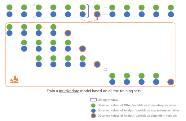
When forecasting to new time steps, each related variable is forecasted using a univariate forest-based forecast, and these forecasted values are used as explanatory variables when forecasting future values of the analysis variable. The results of all forecasts (the analysis variable and all explanatory variables) are stored in the output space-time cube.

Multivariate forecasts are created using time windows.

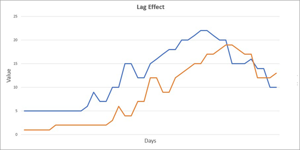
You can also use the Forest-based Forecast tool to estimate and visualize lagged effects between the analysis variable and the other variables. The lag effect is when there is a delay between a change in any other variable and a change in the analysis variable, and it is present in many situations involving time series of multiple variables. For example, spending on advertising often has a lagged effect on sales revenue because people need time to see the advertisements before deciding to purchase. In the previous example of emergency room visits for asthma and pollution levels, there may also be a lag between a rise in pollution levels and a rise in emergency room visits because it may take time for negative health effects to accumulate enough to require emergency care.

The following image shows the lag effect in which changes in the value of the blue time series lag four days behind the orange line:

When a lag is present between any explanatory variables and the analysis variable, you can gain more information about the analysis variable by looking back in time by the length of the lag. For example, if there is a two-week lag between advertising spending and sales revenue, when forecasting sales revenue for a specific day, it is more informative to look at advertising spending two weeks prior compared to the amount spent in the last few days.

The forest model can detect and use the lag effect between variables because the moving time window always forecasts the time step immediately after it. The last value in the time window is always one time step before the forecast; the next to last time step in the time window is always two time steps before the forecast; and so on. Because the time window shifts, each explanatory variable is represented as a separate factor for each time step within the time window, allowing it to compare different explanatory variables at different lags and determine which are most important for forecasting. See How Forest-based Classification and Regression works for more information.

For example, the chart below shows the important time-lagged variables of individual counties in forecasting daily new deaths from coronavirus disease 2019 (COVID-19) in early 2021. The model uses the number of people receiving a vaccine each day as an explanatory variable. The values of the x-axis refer to each time step within the time window, and this image has 14 values because it used a time window of 14 days. The values of the x-axis represent the number of time steps before the forecast, so they go back in time as you move from left to right in the chart. The leftmost value of 1 means that it is one day before the forecast, which corresponds to the final time step in the time window. Similarly, the rightmost value of 14 represents 14 days before the forecast, corresponding to the first time step of the 14-day time window. For each time step, the light- and dark-blue columns represent counts of locations where that factor was determined to be among the most important factors in forecasting new daily deaths from COVID-19, so the larger the count, the more important the factor overall among the locations. The dark-blue bars represent the analysis variable, new deaths from COVID-19, and the bars are highest in the first three to four time lags, indicating that the number of deaths of the previous three to four days is most predictive of deaths the following day. While this data does not demonstrate it, it is possible for a variable to lag itself, such as with cyclical variables like temperature, where looking 24 hours back is more predictive than looking 2 hours back due to day and night cycles. The light-blue bars represent the number of new vaccines administered on the day, and the highest light-blue bars appear 10 to 14 days back in the time window (the bars farthest to the right), indicating that increases or decreases in vaccine counts affect the number of deaths 10 to 14 days in the future. This 10- to 14-day lag corresponds to the time needed to develop peak immunity following a vaccination.

Factors important in forecasting new daily deaths from COVID-19 are displayed. Deaths in the three to four most recent days are most predictive of new deaths. The number of new vaccines administered 10 to 14 days in the past is most predictive of new deaths.

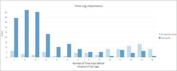
The Time Lag Importance chart is included with the output table produced by the optional Output Importance Table parameter.

For Individual location model scale, the table contains a row for each important variable at each location. The number of factors deemed important at each location depends on the Importance Threshold parameter value. For example, if 15 is provided, the top 15 percent of factors for each location will be included in the table and chart. The default value is 10. To create the table and chart, you must include at least one other variable in the Other Variables parameter. The number of time lags in the table and chart is equal to the value of the Time Step Window parameter, so the time window must be wider than any lagged effects you want to capture. For example, a one-week time window would not be able to capture the lagged effect of vaccines on number of deaths from COVID-19.

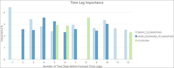
For Entire cube model scale, other variables do not need to be provided to create the table and chart, and the y-axis of the chart is the raw importance percent (rather than a count of locations exceeding a threshold) because all locations share the same forecast model. The following image shows the Time Lag Importance chart for an entire cube analysis with twelve time lags and three variables:

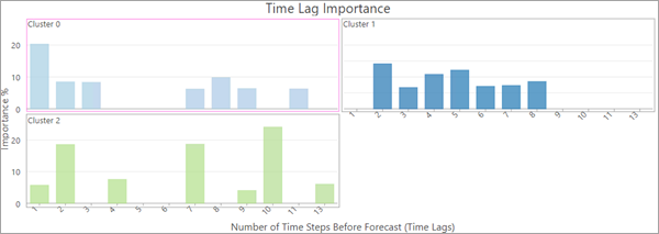
For Time series cluster model scale, the chart is only created if other variables are not provided, and the chart will display a grid of charts separated by cluster. The following image shows the Time Lag Importance for three time series clusters:

Corrections for low variability

If any of the variables used in the analysis at a location do not have sufficient variability, the forest-based forecast model cannot be trained and estimated at that location. If the analysis variable is constant for every time step at a location, the location is excluded from training; the constant value is forecasted at every future time step, and confidence intervals are not included with the forecasts.

If the location has at least two unique values in the time series, two additional checks are performed on the analysis variable and on any other variables. First, for all time steps in the time series, determine the proportion containing a constant value. Second, for only time steps that were not excluded for validation, determine the proportion containing a constant value. If either of these proportions exceeds two-thirds, a small amount of random noise is added to the values to create variability in the time series, and the forecast and validation models are calculated using the new values. The noise added to each time step is a random uniform number between 0 and 0.000001 (1e-6). If the range of the values of the time series is less than 0.001, the noise is uniform between 0 and the range value multiplied by 1e-6.

Even with random added noise, it is still possible for the forest-based model to fail to calculate after 30 attempts. This is most common for very short time series.

Seasonality and choosing a time window

The number of time steps within each time step window is an important choice for the forest model. A major consideration is whether the time series displays seasonality where natural cyclical patterns repeat over a certain number of time steps. For example, temperature displays yearly seasonal cycles according to seasons of the year. Because the time window is used to build associated explanatory and dependent variables, it is most effective when those explanatory variables all come from the same seasonal cycle so that there is as little seasonal correlation between the explanatory variables as possible. It is recommended that you use the number of time steps in a natural season for the length of the time step window. If your data displays multiple seasons, it is recommended that you use the length of the longest season.

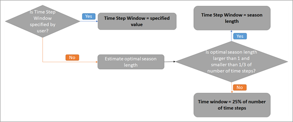
If you know the number of time steps that correspond to one season in your data, you can specify it in the Time Step Window parameter, and this value will be used by every location in the space-time cube. If you do not know the length of a season or if the seasonal length is different for different locations, the parameter value can be left empty, and an optimal season length will be estimated for each location using a spectral density function. For details about this function, see the Additional resources section.

For an individual location, if the optimal season length determined by spectral analysis is greater than one and not greater than one-third of the number of time steps at the location, the time step window is set to this optimal value. Otherwise, the location uses 25 percent (rounded down) of the number of time steps at the location for the time step window. This ensures that there is at least one time step in the window and that at least three full seasonal cycles are used as explanatory variables. The time step value used at the location is saved in the Time Window field of the output features. The Is Seasonal field of the output features will contain the value 1 if the time step window was determined using spectral analysis and will contain 0 otherwise. This workflow is summarized in the following image:

The time step window can be specified or estimated for each location by detecting seasonality.

For the Entire cube and Time series cluster model scales, the default time window is 25 percent (rounded down) of the number of time steps. This is because different locations often have different seasonable behavior (for example, winter begins in some locations earlier than in others), so a single seasonal trend cannot be estimated and shared between all locations in the group.

Approaches to forecasting

There are four ways you can represent the values of the explanatory and dependent variables that will be used to train the forest. These options are specified using the Forecast Approach parameter.

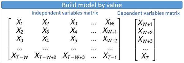
The first option is Build model by value. This option uses the raw values in the space-time bins for the explanatory and dependent variables. When this option is chosen, the forecasted values will be contained within the range of the dependent variables, so you should not use this option if your data has trends where you expect the values to continue to increase or decrease when forecasting the future. The image below shows the sets of variables used to train the model for a single location in which each row displays the set of explanatory variables and the associated dependent variable. T is the number of time steps in the space-time cube, W is the number of time steps in each time step window, and X_t is the raw value of the time series at time t.

Note:

For Entire cube and Time series cluster model scales, Build model by value is the only available forecast approach.

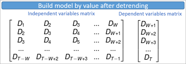
The second option is Build model by value after detrending. This is the default option of the tool. This option performs a first-order (linear) trend removal on the entire time series at each location, and these detrended values are used as the explanatory and dependent variables. Using this option allows the forecasts to follow this trend into the future so that the forecasted values can be estimated outside of the range of the dependent variables. The image below shows the sets of variables used to train the model for a single location in which each row displays the set of explanatory variables and the associated dependent variable. T is the number of time steps in the space-time cube, W is the number of time steps in each time step window, and D_t is the detrended value of the time series at time t.

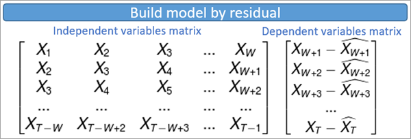
The third option is Build model by residual. This option creates an ordinary least-squares (OLS) regression model to predict the dependent variable based on the explanatory variables within each time window. The residual of this regression model (the difference between the OLS prediction and the raw value of the dependent variable) is used to represent the dependent variable when training the forest. The image below shows the sets of variables used to train the model for a single location in which each row displays the set of explanatory variables and the associated dependent variable. T is the number of time steps in the space-time cube, W is the number of time steps in each time step window, X_t is the value of the time series at time t, and X^{^}_t (X_t-hat) is the value estimated from OLS at time t.

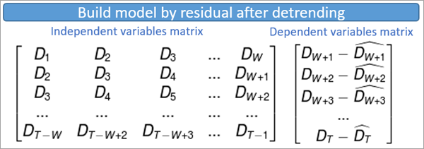
The last option is Build model by residual after detrending. This option first performs a first-order (linear) trend removal on the entire time series at a location. It then builds an OLS regression model to predict the detrended dependent variable based on the detrended explanatory variables within each time window. The residual of this regression model (the difference between the OLS prediction and the detrended value of the dependent variable) is used to represent the dependent variable when training the forest. The image below shows the sets of variables used to train the model for a single location in which each row displays the set of explanatory variables and the associated dependent variable. T is the number of time steps in the space-time cube, W is the number of time steps in each time step window, D_t is the detrended value of the time series at time t, and D^{^}_t (D_t-hat) is the value estimated from OLS at time t.

Construct confidence intervals

If at least two time steps are excluded for validation, the tool calculates 90 percent confidence intervals for each forecasted time step that appear as fields in the output features and display in the pop-up charts described in the Tool outputs section. The tool constructs the confidence intervals by estimating the standard error of each forecasted value and creating confidence bounds 1.645 standard errors above and below each forecasted value.

The tool performs the following calculations to estimate the standard errors:

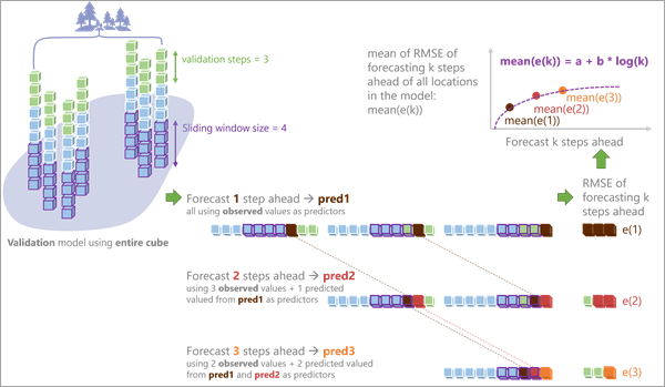
1. Calculate the Validation RMSE of one-step-ahead forecasts using time windows of size T to predict the time steps excluded for validation. The one-step-ahead Validation RMSE can only be calculated with time windows that were not used to train the forecast model and that have at least one time step after the window to predict. The first time window is the final T time steps before the excluded time steps, and it predicts the first excluded time step. The second time window is the final (T-1) time steps and the first excluded time step (the value is returned to be used to calculate the RMSE), and it predicts the second excluded time step. The final time window predicts the final excluded time steps using the previous T time steps (returned to the dataset). For individual location model scale, the one-step-ahead forecast calculates the RMSE using M values, for M time steps withheld for validation. For entire cube or time series cluster model scales, each location in the group contributes M values to the one-step-ahead RMSE calculation.
2. Calculate the Validation RMSE of two-step-ahead forecasts also using time windows within the excluded time steps. Each window uses the predicted value from step 1 as the final time step to predict the next excluded time step. For two-step-ahead forecasts, each location contributes (M-1) values to the two-step-ahead RMSE calculation.
3. Calculate the Validation RMSE of K-step-ahead forecasts, up to K=M. Each location uses the predicted values from the (K-1)-step-ahead RMSE calculations and contributes (M-K+1) values in the RMSE calculation. The final M-step-ahead RMSE calculation uses one value per location.
4. Fit a regression model predicting the mean K-step-ahead RMSE of the locations in the group (or individual location) using log(K) as an explanatory variable. Use this model to estimate the standard errors for all future time steps (all values of K), including the first M forecasted values.

The following image illustrates this process for an entire cube analysis with three time steps (M=3) withheld for validation and a time window of four time steps (T=4).

Confidence intervals are estimated for the forecasts of an entire cube.

Note:

In some cases, the estimated slope or intercept of the regression model predicting the standard errors can be negative. If the estimated intercept is negative, the model is fit without an intercept. If the slope is negative, the maximum RMSE among the withheld time steps (individual location, time series cluster, or entire cube) is used as the standard error of all forecasted values.

Identifying time series outliers

Outliers in time series data are values that significantly differ from the patterns and trends of the other values in the time series. For example, large numbers of online purchases around holidays or high numbers of traffic accidents during heavy rainstorms would likely be detected as outliers in their time series. Simple data entry errors, such as omitting the decimal of a number, are another common source of outliers. Identifying outliers in time series forecasting is important because outliers influence the forecast model that is used to forecast future values, and even a small number of outliers in the time series of a location can significantly reduce the accuracy and reliability of the forecasts. Locations with outliers, particularly outliers toward the beginning or end of the time series, may produce misleading forecasts, and identifying these locations helps you determine how confident you should be in the forecasted values at each location.

Outliers are not determined simply by their raw values but instead by how much their values differ from the fitted values of the forecast model. This means that whether or not a value is determined to be an outlier is contextual and depends both on its place and time. The forecast model defines what the value is expected to be based on the entire time series, and outliers are the values that deviate significantly from this baseline. For example, consider a time series of annual mean temperature. Because average temperatures have increased over the last several decades, the fitted forecast model of temperature will also increase over time to reflect this increase. This means that a temperature value that would be considered typical and not an outlier in 1950 would likely be considered an outlier if the same temperature occurred in 2020. In other words, a typical temperature from 1950 would be considered very low by the standards of 2020.

You can choose to detect time series outliers at each location using the Identify Outliers parameter. If specified, the Generalized Extreme Studentized Deviate (ESD) test is performed for each location to test for time series outliers. The confidence level of the test can be specified with the Level of Confidence parameter, and 90 percent confidence is used by default. The Generalized ESD test iteratively tests for a single outlier, two outliers, three outliers, and so on, at each location up to the value of the Maximum Number of Outliers parameter (by default, 5 percent of the number of time steps, rounded down), and the largest statistically significant number of outliers is returned. The number of outliers at each location can be seen in the attribute table of the output features, and individual outliers can be seen in the time series pop-up charts that are discussed in the next section.

Learn more about outliers in time series analysis, the Generalized ESD test, and how to interpret the results

Tool outputs

The primary output of the tool is a 2D feature class showing each location in the Input Space Time Cube value symbolized by the final forecasted time step with the forecasts for all other time steps stored as fields. Although each location is independently forecasted and spatial relationships are not taken into account, the map may display spatial patterns for areas with similar time series.

Pop-up charts

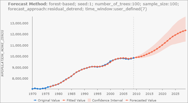
Clicking any feature on the map using the Explore navigation tool displays a chart in the Pop-up pane showing the values of the space-time cube along with the fitted forest model and the forecasted values along with 90 percent confidence intervals for each forecast. The values of the space-time cube are displayed in blue and are connected by a blue line. The fitted values are displayed in orange and are connected by a dashed orange line. The forecasted values are displayed in orange and are connected by a solid orange line representing the forecasting of the forest model. Light red confidence bounds are drawn around each forecasted value. You can hover over any point in the chart to see the date and value of the point. Additionally, if you chose to detect outliers in time series, any outliers are displayed as large purple dots.

The pop-up chart displays the original values, fitted values, forecasted values, and confidence intervals.

Note:

Pop-up charts are not created when the output features are saved as a shapefile (.shp). Additionally, if the confidence intervals extend off the chart, a Show Full Data Range button appears above the chart that allows you to extend the chart to show the entire confidence interval.

Geoprocessing messages

The tool provides a number of messages with information about the tool execution. The messages have three main sections.

The Input Space Time Cube Details section displays properties of the input space-time cube along with information about the number of time steps, number of locations, and number of space-time bins. The properties displayed in this first section depend on how the cube was originally created, so the information varies from cube to cube.

The Analysis Details section displays properties of the forecast results, including the number of forecasted time steps, the number of time steps excluded for validation, the percent of locations where seasonality was detected by spectral analysis, and information about the forecasted time steps. If a value is not provided for the Time Step Window parameter, summary statistics of the estimated time step window are displayed, including the minimum, maximum, average, median, and standard deviation.

The Summary of Accuracy across Locations section displays summary statistics for the Forecast RMSE and Validation RMSE among all of the locations. For each value, the minimum, maximum, mean, median, and standard deviation is displayed.

The Summary of Time Series Outliers section appears if you choose to detect time series outliers using the Outlier Option parameter. This section displays information including the number and percent of locations containing outliers, the time step containing the most outliers, and summary statistics for the number of outliers by location and by time step.

Note:

Geoprocessing messages appear at the bottom of the Geoprocessing pane during tool execution. You can access the messages by hovering over the progress bar, clicking the pop-out button , or expanding the messages section in the Geoprocessing pane. You can also access the messages for a previously run tool using geoprocessing history.

Fields of the output features

In addition to Object ID, geometry fields, and the field containing the pop-up charts, the Output Features will have the following fields:

• Location ID (LOCATION)—The Location ID of the corresponding location of the space-time cube.
• Forecast for (Analysis Variable) in (Time Step) (FCAST_1, FCAST_2, and so on)—The forecasted value of each future time step. The field alias displays the name of the Analysis Variable and the date of the forecast. A field of this type is created for each forecasted time step.
• High Interval for (Analysis Variable) in (Time Step) (HIGH_1, HIGH_2, and so on)—The upper bound of a 90 percent confidence interval for the forecasted value of each future time step. The field alias displays the name of the Analysis Variable and the date of the forecast. A field of this type is created for each forecasted time step.
• Low Interval for (Analysis Variable) in (Time Step) (LOW_1, LOW_2, and so on)—The lower bound of a 90 percent confidence interval for the forecasted value of each future time step. The field alias displays the name of the Analysis Variable and the date of the forecast. A field of this type is created for each forecasted time step.
• Forecast Root Mean Square Error (F_RMSE)—The Forecast RMSE.
• Validation Root Mean Square Error (V_RMSE)—The Validation RMSE. If no time steps were excluded for validation, this field is not created.
• Time Window (TIMEWINDOW)—The time step window used at the location.
• Is Seasonal (IS_SEASON)—A Boolean variable indicating whether the time step window at the location was determined by spectral density. A value of 1 indicates seasonality was detected by spectral density, and a value of 0 indicates no seasonality was detected. If a value is specified in the Time Window parameter, all locations have the value 0 in this field.
• Forecast Method (METHOD)—A text field displaying the parameters of the forest model, including the random seed, number of trees, sample size, forecast approach, whether the time step window was specified by the user or determined by the tool, any other variables, and information about model scale and cluster variability (if applicable). This field can be used to reproduce results, and it allows you to identify which models are used in the Evaluate Forecasts By Location tool.
• Number of Model Fit Outliers (N_OUTLIERS)—The number of outliers detected in the time series of the location. This field is only created if you chose to detect outliers with the Outlier Option parameter.

Output space-time cube

If an Output Space Time Cube is specified, the output cube contains all of the original values from the input space-time cube with the forecasted values appended. This new space-time cube can be displayed using the Visualize Space Time Cube in 2D or Visualize Space time Cube in 3D tools and can be used as input to the tools in the Space Time Pattern Mining toolbox, such as Emerging Hot Spot Analysis and Time Series Clustering.

Multiple forecasted space-time cubes can be compared and merged using the Evaluate Forecasts by Location tool. This allows you to create multiple forecast cubes using different forecasting tools and parameters, and the tool identifies the best forecast for each location using either Forecast or Validation RMSE.

Best practices and limitations

When deciding whether this tool is appropriate for your data and which parameters to use, consider the following:

• Compared to other forecasting tools in the Time Series Forecasting toolset, this tool is the most complicated but makes the fewest assumptions about the data. It is recommended for time series with complicated shapes and trends that are difficult to model with simple or smooth mathematical functions. It is also recommended when the assumptions of other methods are not satisfied.
• This tool can be used to explore different model scales and the interactions between different time series variables. It is recommended that you run the tool multiple times with different scales and other variables, and use the Evaluate Forecasts By Location tool to decide the best forecasts for each location.

• Deciding on the value of the Number of Time Steps to Exclude for Validation parameter is important. The more time steps that are excluded, the fewer time steps remain to estimate the validation model. However, if too few time steps are excluded, the Validation RMSE is estimated using a small amount of data and may be misleading. It is recommended that you exclude as many time steps as possible while still maintaining sufficient time steps to estimate the validation model. It is also recommended that you withhold at least as many time steps for validation as the number of time steps you intend to forecast, if your space-time cube has enough time steps to allow this.

  Additionally, building confidence intervals for the forecasted values requires fitting a regression function to the time steps withheld for validation. Because at least two values are required to fit this function, at least two time steps must be withheld to create confidence intervals of the forecasts. However, the regression function will be more accurate (resulting in more accurate confidence intervals) for a larger number of withheld time steps. For the most accurate confidence intervals, it is recommended that you withhold at least the default value of 10 percent of the time steps for validation.

• This tool may produce unstable and unreliable forecasts when the same value is repeated many times within the time series. A common source of repeated identical values is zero-inflation, in which your data represents counts and many of the time steps have the value 0.
• If you choose to identify outliers, it is recommended that you provide a value for the Time Step Window parameter rather than leaving the parameter empty and estimating a different time step window at each location. For each location, the forest model uses the time steps in the first time step window to train the forecast model, and outliers are only detected for the remaining time steps. If different locations exclude different numbers of time steps for training, summary statistics such as the mean, minimum, and maximum number of outliers per time step or per location may be misleading. These statistics are calculated only for time steps that were included at every location.

Additional resources

For more information about forest models, see the following references:

• Breiman, Leo. (2001). "Random Forests." Machine Learning 45 (1): 5-32. https://doi.org/10.1023/A:1010933404324.
• Breiman, L., J.H. Friedman, R.A. Olshen, and C.J. Stone. (2017). Classification and regression trees. New York: Routledge. Chapter 4.

For additional resources and references for forest models, see How Forest-based Classification and Regression works.

For more information about the spectral density function used to estimate the length of time windows, see the findfrequency function in the following references:

• Hyndman R, Athanasopoulos G, Bergmeir C, Caceres G, Chhay L, O'Hara-Wild M, Petropoulos F, Razbash S, Wang E, and Yasmeen F (2019). "Forecasting functions for time series and linear models." R package version 8.7, https://pkg.robjhyndman.com/forecast.
• Hyndman RJ and Khandakar Y (2008). "Automatic time series forecasting: the forecast package for R." Journal of Statistical Software, 26(3), pp. 1-22. https://www.jstatsoft.org/article/view/v027i03.

For more information about including explanatory variables and the lag effect, see the following reference:

• Zheng, H., and Kusiak, A. (2009). "Prediction of Wind Farm Power Ramp Rates: A Data-Mining Approach." ASME. J. Sol. Energy Eng, 131(3): 031011. https://doi.org/10.1115/1.3142727.