Location-allocation analysis layer

This topic describes the location allocation analysis layer's feature classes and analysis properties.

Learn more about the location-allocation solver

Facilities feature class

The Facilities feature class stores the network locations used as the candidate locations from which the actual locations will be chosen from in location-allocation analyses. When a new location-allocation analysis layer is created, the Facilities class is empty. It is populated only when network locations are added into it. A minimum of one facility and one demand point is necessary to solve the analysis.

Facilities: Input fields

Input field	Description
ObjectID	The system-managed ID field.
Shape	The geometry field indicating the geographic location of the network analysis object.
Name	The name of the network analysis object.
FacilityType	This property specifies whether the facility is a candidate, required, competitor, or chosen facility. It is constrained by a domain of values, which is referenced by the integer value in parentheses in the following list: Candidate (0)—A candidate facility is a facility that may be part of the solution. Required (1)—A required facility is a facility that must be part of the solution. Competitor (2)—A competitor facility is specific to the Maximize Market Share and Target Market Share problem types. It is a facility that represents your rivals and will remove demand from the problem. Chosen (3)—Once the location-allocation solver determines that a candidate facility is part of the solution, the solver changes the FacilityType value from Candidate to Chosen. If the FacilityType is set to Chosen before solving, the facility is treated as a candidate facility at solve time.
Weight	The relative weighting of the facility, which is used to rate the attractiveness, desirability, or bias of one facility compared to another. For example, a value of 2.0 could capture the preference of customers who prefer, at a ratio of 2 to 1, shopping in one facility over another facility. Example factors that potentially affect facility weight include square footage, neighborhood, and age of the building. Weight values other than 1 are only honored by the Maximize Market Share and Target Market Share problem types.
Capacity	The Capacity property is specific to the Maximize Capacitated Coverage problem type; the other problem types ignore Capacity. This property specifies how much weighted demand the facility is capable of supplying. Excess demand won't be allocated to a facility even if that demand is within the facility's impedance cutoff. Any value assigned to this facility property overrides the network analysis layer's default capacity.
Network location fields SourceID SourceOID PosAlong SideOfEdge SnapX SnapY SnapZ DistanceToNetworkInMeters	Together, these properties describe the point on the network where the object is located. Learn more about locating inputs on a network
CurbApproach	The CurbApproach field specifies the direction a vehicle may arrive at and depart from the network location. The shortest path between two points can change depending on the direction of travel permitted when arriving at or departing from a location. There are four choices (their coded values are shown in parentheses): Either side of vehicle (0)—The vehicle can approach and depart the point in either direction. U-turns are allowed. Choose this setting if a vehicle can make a U-turn at the location or if it can pull into a driveway or parking lot and turn around. Right side of vehicle (1)—When the vehicle approaches and departs the point, the curb must be on the right side of the vehicle. A U-turn is prohibited. Left side of vehicle (2)—When the vehicle approaches and departs the point, the curb must be on the left side of the vehicle. A U-turn is prohibited. No U-Turn (3)—When the vehicle approaches the point, the curb can be on either side of the vehicle; however, the vehicle must depart without turning around. Learn more about U-turns and curb approach For location-allocation analyses, the No U-turn (3) value functions the same as Either side of vehicle (0).

Facilities: Input/output fields

Input/Output field

Description

Status

Indicates the status of the point with respect to its location on the network and the outcome of the analysis. The possible values are the following: 0 (OK)—The point was located on the network. 1 (Not Located)—The point was not located on the network and consequently was not included in the analysis. 2 (Network element not located)—The network element identified by the point's network location fields can't be found. This can occur when a network element where the point should be was deleted, and the network location was not recalculated. 3 (Element not traversable)—The network element that the point is located on is not traversable. This can occur when the element is restricted by a restriction attribute. 4 (Invalid Field Values)—Field values fall outside a range or coded-value domain. For example, a negative number exists where positive numbers are required. 5 (Not Reached)—The point can't be reached by the solver. The point may be on a separate, disconnected area of the network from the other inputs, or barriers or restrictions prevent travel to or from the point. 6 (Time window violation)—The point could not be reached within the designated time windows. This status only applies to network analysis types that support time windows. 7 (Not located on closest)—The closest network location to the point is not traversable because of a restriction or barrier, so the point has been located on the closest traversable network feature instead.

Facilities: Output fields

Output field	Description
DemandCount	This field contains a count of demand points allocated to the facility. A nonzero value means the facility was chosen as part of the solution.
DemandWeight	This field contains a sum of the effective weight from all demand points allocated to the facility. The value is a sum of all the Weight values from the demand points allocated to the facility. In the case of the Maximize Attendance and Maximize Market Share problem types, the value is an apportioned sum of the Weight field values, since these problem types allow demand to decay with distance or be split among many facilities.
Total_[Cost] (for instance Total_Miles, where Miles is the travel cost)	This field contains a sum of network costs between the facility and each of the demand points allocated to the facility. The [Impedance] portion of the field name is replaced with the network attribute name, for example, Total_Meters, where Meters is the name of the network attribute.
TotalWeighted_[Cost] (for instance, TotalWeighted_Miles, where Miles is the travel cost)	This field stores the cumulative weighted cost for a facility. The weighted cost for a demand point is its weight multiplied by the least-cost path between the facility and the demand point. The weighted cost for a facility is the sum of all the weighted costs of demand points allocated to the facility. For example, if a demand point with a weight of two is allocated to a facility 10 miles away, the TotalWeighted_Miles value is 20 (2 x 10). If another demand point with a weight of three is allocated to the same facility and is 5 miles away, the TotalWeighted_Miles value increases to 35 (3 x 5 + 20).

Demand Points feature class

The Demand Points feature class stores demand points that are part of a given location-allocation analysis layer. A demand point is typically a location that represents the people or things requiring the goods and services your facilities provide. A demand point could be a ZIP Code centroid weighted by the number of people residing within it or by the expected consumption generated by those people. Demand points could also represent business customers. If you supply businesses with a high turnover of inventory, they would be weighted more heavily than those with a low turnover rate.

Demand points can override the distance cutoff for the location-allocation problem type. This is useful if some demand points have different needs or behavior. For instance, when prepositioning ambulances, it may be acceptable to reach everyone within four minutes, except for areas with a high-density of elderly people, such as senior centers, which require a faster response time of two minutes.

Demand Points: Input fields

Input field	Description
ObjectID	The system-managed ID field.
Shape	The geometry field indicating the geographic location of the network analysis object.
Name	The name of the network analysis object.
GroupName	The name of the group the demand point is part of. This property is ignored for the Maximize Capacitated Coverage, Target Market Share, and Maximize Market Share problem types. If demand points share a group name, the solver allocates all members of the group to the same facility. Minimizing distance without grouped demand points Minimizing distance with grouped demand points. In this example, the yellow demand points have the same GroupName value, so they are allocated to the same facility. If constraints, such as a cutoff distance, prevent any of the demand points in the group from reaching the same facility, none of the demand points are allocated.
Weight	The relative weighting of the demand point. A value of 2.0 means the demand point is twice as important as one with a weight of 1.0.
ImpedanceTransformation	Any value assigned to this demand point property overrides the network analysis layer's impedance transformation value.
ImpedanceParameter	Any value assigned to this demand point property overrides the network analysis layer's impedance parameter value.
Cutoff_[Cost] (for instance Cutoff_Miles, where Miles is the travel cost)	Any value assigned to this demand point property overrides the network analysis layer's Cutoff value.
Network location fields SourceID SourceOID PosAlong SideOfEdge SnapX SnapY SnapZ DistanceToNetworkInMeters	Together, these properties describe the point on the network where the object is located.
CurbApproach	The CurbApproach field specifies the direction a vehicle may arrive at and depart from the network location. The shortest path between two points can change depending on the direction of travel permitted when arriving at or departing from a location. There are four choices (their coded values are shown in parentheses): Either side of vehicle (0)—The vehicle can approach and depart the point in either direction. U-turns are allowed. Choose this setting if a vehicle can make a U-turn at the location or if it can pull into a driveway or parking lot and turn around. Right side of vehicle (1)—When the vehicle approaches and departs the point, the curb must be on the right side of the vehicle. A U-turn is prohibited. Left side of vehicle (2)—When the vehicle approaches and departs the point, the curb must be on the left side of the vehicle. A U-turn is prohibited. No U-Turn (3)—When the vehicle approaches the point, the curb can be on either side of the vehicle; however, the vehicle must depart without turning around. Learn more about U-turns and curb approach For location-allocation analyses, the No U-turn (3) value functions the same as Either side of vehicle (0).

Demand Points: Input/output fields

Input/output field

Description

Status

Indicates the status of the point with respect to its location on the network and the outcome of the analysis. The possible values are the following: 0 (OK)—The point was located on the network. 1 (Not Located)—The point was not located on the network and consequently was not included in the analysis. 2 (Network element not located)—The network element identified by the point's network location fields can't be found. This can occur when a network element where the point should be was deleted, and the network location was not recalculated. 3 (Element not traversable)—The network element that the point is located on is not traversable. This can occur when the element is restricted by a restriction attribute. 4 (Invalid Field Values)—Field values fall outside a range or coded-value domain. For example, a negative number exists where positive numbers are required. 5 (Not Reached)—The point can't be reached by the solver. The point may be on a separate, disconnected area of the network from the other inputs, or barriers or restrictions prevent travel to or from the point. 6 (Time window violation)—The point could not be reached within the designated time windows. This status only applies to network analysis types that support time windows. 7 (Not located on closest)—The closest network location to the point is not traversable because of a restriction or barrier, so the point has been located on the closest traversable network feature instead.

Demand Points: Output fields

Output field	Description
FacilityID	The ObjectID of the facility the demand point was allocated to. If the value is null, the demand point was not allocated to a facility, or it was allocated to more than one facility; the latter is only possible in the market share problem types.
AllocatedWeight	This is the amount of demand allocated to chosen and required facilities. The value excludes demand allocated to competing facilities. The value can have three interpretations: A null value indicates the demand point wasn't assigned to any facility. This can result, for example, if the demand point is outside all impedance cutoffs or the demand point is on a restricted network element. A zero value indicates the demand point is only assigned to competing facilities. A positive, nonzero value indicates how much demand is assigned to your chosen and required facilities.

Lines feature class

The Lines feature class is an output-only network analysis class containing line features generated by the solver during the solve operation. It contains line features that connect demand points to the facilities to which they are allocated. If a demand point is allocated to more than one facility, it has one line for each facility to which it is allocated. If a demand point is not allocated to any facility, it won't have any corresponding lines. Location-allocation output in the Lines feature class can either be represented on the map as straight lines or not displayed in the map at all; either way, the analysis always considers the shortest network path between the facility and the demand point; thus, the cost-related attributes reflect network costs, not straight-line distances. The reason the actual shape of the network paths are not output is that they are rarely needed in location-allocation, and generating the shape of the paths would require a substantial increase in the solve time and potentially exhaust your system's resources, especially for large problems.

Lines: Output fields

Output field	Description
ObjectID	The system-managed ID field.
Shape	The geometry field indicating the geographic location of the network analysis object. If the Output Geometry Linear Shape Type property of the analysis layer is set to No Lines, no shape is returned. Setting the Output Geometry Linear Shape Type property to Straight Lines returns straight lines that connect each demand-point or facility pair.
Name	The name of the line. Names are formatted so the facility name and the demand point name are listed in the order they are visited. When the travel direction of the network analysis layer is set to Away from facilities, the name format is [facility name] - [demand point name]; it is [demand point name] - [facility name] when the property is set to Toward facilities.
FacilityID	The unique ID of the facility with which the line is associated. A line is always associated with one facility and one demand point.
DemandID	The unique ID of the demand point with which the line is associated. A line is always associated with one facility and one demand point.
Weight	The weight assigned from the connected demand point (DemandID) to the connect facility (FacilityID).
TotalWeighted_[Cost] (for instance, TotalWeighted_Miles, where Miles is the travel cost)	The weighted cost of traveling between the facility and the demand point. This is the Total_[Cost] value multiplied by the weight of the demand point allocated to the facility. The active cost attribute will have an accompanying Total_[Cost] field, but the accumulated cost attributes won't. If you need to calculate weighted impedance for accumulated attributes, you can multiply the values from the Weight and appropriate Total_[Cost] fields. Note that though the lines have either straight or null geometries, the impedance always refers to network costs, not straight-line distances.
Total_[Cost] (for instance Total_Miles, where Miles is the travel cost)	The network cost of traveling between the facility and the demand point. All accumulated attributes, as well as the active cost attribute, will have an accompanying Total_[Cost] field. Note that though the lines have either straight or null geometries, the cost always refers to network costs, not straight-line distances.

Location-allocation analysis layer properties

The following subsections list parameters that you can set on the analysis layer. They are found on the Location-Allocation Layer tab, which is available only if your Location-allocation layer or one of its sublayers is selected in the Contents pane.

Analysis

Use the options in this section to estimate the credits and run the analysis.

Run

Once you load input features and set analysis properties, click the Run button to run the analysis. If the analysis uses credits, and the number of credits estimated for the solve exceeds the available credits, you will see an error message that blocks the solve or a warning message that will allow you to choose whether to proceed with the solve.

The run button may appear different based on the source of the network dataset.

• —The network analysis layer is referencing a local network data source.
• —The network analysis layer is referencing a network data source in ArcGIS Online.
• —The network analysis layer is referencing a network data source in an enterprise portal.

Estimate Credits

The Estimate Credits button can be used to estimate the number of service credits that will be consumed by running the analysis on the selected network analysis layer. When this button is enabled, it indicates that the network analysis layer will consume credits when solved.

The Estimate Credits button is enabled when the following occur:

• The network analysis layer's network data source is hosted in ArcGIS Online.
• Your ArcGIS Enterprise portal routing services are configured from ArcGIS Online.

The Estimate Credits button is disabled when the following occur:

• The network analysis layer's network data source is stored on a local machine.
• You're using your own services published on your ArcGIS Enterprise portal.

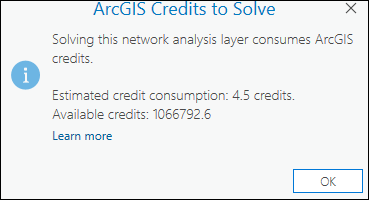
When you click the Estimate Credits button, a dialog box appears with an estimate of how many credits are likely to be consumed solving the current analysis. The credit is estimated based on the number of input locations used in the analysis. The actual credits consumed may change based on the output generated by the Solve operation. Depending on how your organization has set up the credit budgeting and allocation settings, the available credits may not be shown. Also, credit estimation may not always be possible if the network data source is an ArcGIS Enterprise portal with routing services configured from ArcGIS Online.

Learn more about the credit usage by each analysis type

Note:

Depending on the configuration of the ArcGIS Online organization account and the signed-in user, solving the analysis may be blocked or may show a warning if the estimated credits exceed the available credits.

Input Data

Use the options in this section to import the input features to participate in the analysis.

Import Facilities

Use Import Facilities to load features from another data source, such as a point feature layer, into the Facilities feature class.

Import Demand Points

Use Import Demand Points to load features from another data source, such as a point feature layer, into the Demand Points feature class.

Import Barriers

Use the Import Point Barriers , Import Line Barriers , or Import Polygon Barriers buttons to load features from another data source, such as another feature layer, into one of the barriers feature classes (point barriers, line barriers, or polygon barriers).

Create Features

Use the Create Features button to open the Create Features pane. Select from the available templates to create features in the current map.

Travel Settings

Use the options in the Travel Settings section to select the travel mode.

Mode

The Mode drop-down list allows you to choose a travel mode, which is a group of settings that together model the movement of pedestrians, cars, trucks, or another travel mode. The choices available in the drop-down list depend on the travel modes that are configured on the network data source that the network analysis layer is referencing.

Direction

Your location-allocation analysis can accumulate travel time or other cost in the direction away from or toward the facilities.

• Away from facilities —The direction of travel is from the facility to the demand point.
• Toward facilities —The direction of travel is from the demand point to the facility.

On a network with one-way restrictions and different travel times based on direction of travel, changing the travel direction can produce different results. The direction you should choose depends on the nature of your analysis. For example, to route the closest fire truck (the facility) to the location of a fire (the incident), the Away from facilities option is the most appropriate choice. Alternatively, to identify the closest gas station (facility) to your current location, Toward facilities is a better choice because you need to travel to the facility.

Cutoff

When calculating the least-cost path from a facility to a demand point, the location-allocation solver will stop searching for demand points that lie beyond this impedance cutoff. No demand points beyond this limit will be found for that facility. The units you should use for the cutoff value are shown next to the Mode drop-down arrow.

Accumulate Cost Attributes

The Accumulate Cost Attributes drop-down menu can be used to configure accumulated cost attributes. The drop-down menu is unavailable if the network data source is a service, the output geometry types do not include lines, or there are no cost attributes. The attributes are grouped by unit domain shown as the group header (for example, Time or Distance). A checked check box indicates that the analysis layer will accumulate the checked attribute during the solve.

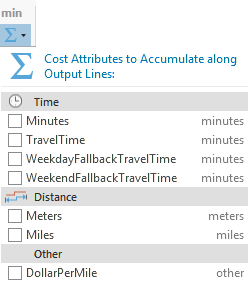
When multiple analysis layers of the same layer type are selected, the check box shows a mixed state if all layers do not share the same checked status for one attribute. In the following image, the WeekendFallbackTravelTime attribute is selected for multiple layers, so it has a check mark.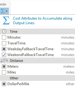

If all selected layers share the checked status for an attribute, the check box shows that state.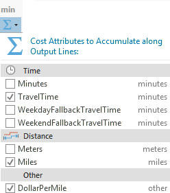

Facilities

You can specify the number of facilities to find per incident by entering a value for Facilities or use the controls to specify a value.

Note:

The Facilities option is disabled for Maximize Coverage and Minimize facilities and the Target Market Share problem types.

Problem type

Use the controls in this section to select the problem and cost transformation function type for modeling the relationship between demand points and facilities.

Type

The Type drop-down menu allows you to specify the problem type solved by the location-allocation solver.

Problem type	Description
Minimize Weighted Impedance (P-Median)	Facilities are located such that the sum of all weighted costs between demand points and solution facilities is minimized. The arrows in the graphic below highlight the fact that allocation is based on distance among all demand points. Minimize Weighted Impedance (P-Median) chooses facilities such that the sum of weighted impedances (demand allocated to a facility multiplied by the impedance to the facility) is minimized. This problem type is traditionally used to locate warehouses, because it can reduce the overall transportation costs of delivering goods to outlets. Since Minimize Weighted Impedance (P-Median) reduces the overall distance the public needs to travel to reach the chosen facilities, the minimize impedance problem without an impedance cutoff is ordinarily regarded as more equitable than other problem types for locating some public-sector facilities such as libraries, regional airports, museums, department of motor vehicles offices, and health clinics. The following list describes how the minimize weighted impedance problem type handles demand: If an impedance cutoff is set, any demand outside all the facilities' impedance cutoffs is not allocated. A demand point inside the impedance cutoff of one facility has all its demand weight allocated to that facility. A demand point inside the impedance cutoff of two or more facilities has all its demand weight allocated to the nearest facility only.
Maximize Coverage	Facilities are located such that as many demand points as possible are allocated to solution facilities within the impedance cutoff. Maximize Coverage chooses facilities such that as much demand as possible is covered by the impedance cutoff of facilities. In this graphic, the solver was directed to choose three facilities. Maximize Coverage is frequently used to locate fire stations, police stations, and ERS centers, because emergency services are often required to arrive at all demand points within a specified response time. Note that it is important for all organizations, and critical for emergency services, to have accurate and precise data so analysis results correctly model real-world results. Pizza delivery businesses, as opposed to eat-in pizzerias, try to locate stores where they can cover the most people within a certain drive time. People who order pizzas for delivery don't typically worry about how far away the pizzeria is; they are mainly concerned with the pizza arriving within an advertised time window. Therefore, a pizza-delivery business would subtract pizza-preparation time from its advertised delivery time and solve a maximize coverage problem to choose the candidate facility that would capture the most potential customers in the coverage area. (Potential customers of eat-in pizzerias are more affected by distance, since they need to travel to the restaurant; thus, the attendance maximizing or market share problem types would better suit eat-in restaurants.) The following list describes how the Maximize Coverage problem handles demand: Any demand point outside all the facilities' impedance cutoffs is not allocated. A demand point inside the impedance cutoff of one facility has all its demand weight allocated to that facility. A demand point inside the impedance cutoff of two or more facilities has all its demand weight allocated to the nearest facility only.
Maximize Capacitated Coverage	Facilities are located such that as many demand points as possible are allocated to solution facilities within the impedance cutoff; additionally, the weighted demand allocated to a facility can't exceed the facility's capacity. Maximize Capacitated Coverage chooses facilities such that all or the greatest amount of demand can be served without exceeding the capacity of any facility. In this graphic, each facility has a capacity of one, and the solver was directed to choose three facilities. Although the demand point on the bottom of the map is within the impedance cutoff of a facility, it's not allocated, because doing so would surpass a facility's capacity. Maximize Capacitated Coverage behaves like either the Minimize Weighted Impedance (P-Median) or Maximize Coverage problem type but with the added constraint of capacity. (If Cutoff is not set, it behaves like a capacitated version of Minimize Weighted Impedance (P-Median).) You can specify a capacity for a facility by assigning a numeric value to its Capacity property. If a value is not assigned in the Capacity field in the Facilities sublayer for a specific facility, the facility is assigned a capacity from the Capacity property of the Location-Allocation Layer tab. Cases for Maximize Capacitated Coverage include creating territories that encompass a given number of people or businesses, locating hospitals or other medical facilities with a limited number of beds or patients who can be treated, or locating warehouses whose inventory isn't assumed to be unlimited. The following list describes how the Maximize Capacitated Coverage problem handles demand: Unlike Maximize Coverage, Maximize Capacitated Coverage doesn't require an impedance cutoff; however, when an impedance cutoff is specified, any demand point outside all the facilities' impedance cutoffs is not allocated. An allocated demand point has all or none of its demand weight assigned to a facility; that is, demand isn't apportioned with this problem type. If the total demand within the impedance cutoff of a facility is greater than the capacity of the facility, only the demand points that maximize total captured demand and minimize total weighted impedance are allocated. Note: You may notice an apparent inefficiency when a demand point is allocated to a facility that isn't the nearest solution facility. This may occur when demand points have varying weights and when the demand point in question is covered by more than one facility's impedance cutoff (or there are no impedance cutoffs at all). This kind of result indicates the nearest solution facility didn't have adequate capacity for the weighted demand, or the most efficient solution for the entire problem required one or more local inefficiencies. In either case, the solution is correct.
Maximize Coverage and Minimize Facilities	Facilities are located such that as many demand points as possible are allocated to solution facilities within the impedance cutoff; additionally, the number of facilities required to cover demand points is minimized. Maximize Coverage and Minimize Facilities chooses facilities such that as many demand points as possible are within the impedance cutoff of facilities. Additionally, the number of facilities required to cover all demand points is minimized. In this graphic, the solver was able to cover all demand points with only two facilities. Maximize Coverage and Minimize Facilities is the same as Maximize Coverage but with the exception of the number of facilities to locate, which in this case is determined by the solver. When the cost of building facilities is not a limiting factor, the same kinds of organizations that use Maximize Coverage (emergency response, for instance) use Maximize Coverage and Minimize Facilities so all possible demand points will be covered. Maximize Coverage and Minimize Facilities is also used to choose school bus stops when students are required to walk a certain distance before another school bus stop is provided closer to the student's residence. The following list describes how the Maximize Coverage and Minimize Facilities problem handles demand: Any demand point outside all the facilities' impedance cutoffs is not allocated. A demand point inside the impedance cutoff of one facility has all its demand weight allocated to that facility. A demand point inside the impedance cutoff of two or more facilities has all its demand weight allocated to the nearest facility only.
Maximize Attendance	Facilities are chosen such that as much demand weight as possible is allocated to facilities while assuming the demand weight decreases in relation to the distance between the facility and the demand point. Maximize Attendance chooses facilities such that as much demand weight as possible is allocated to facilities while assuming the demand weight decreases with distance. The demand points, represented by pie charts in this graphic, show how much of their total demand is captured by the facility. Specialty stores that have little or no competition benefit from this problem type, but it may also be beneficial to general retailers and restaurants that don't have the data on competitors necessary to perform market share problem types. Some businesses that might benefit from this problem type include coffee shops, fitness centers, dental and medical offices, bowling alleys, and electronics stores. Public transit bus stops are often chosen with the help of Maximize Attendance. Maximize Attendance assumes that the farther people have to travel to reach a facility, the less likely they are to use it. This is reflected in how the amount of demand allocated to facilities diminishes with distance. You specify the distance decay with the impedance transformation. The following list describes how the Maximize Attendance problem handles demand: Demand outside the impedance cutoff of all facilities is not allocated to any facility. When a demand point is inside the impedance cutoff of one facility, its demand weight is partially allocated according to the cutoff and impedance transformation. The demand points in the graphic above have pie charts to represent the ratio of their total demand weight captured by the chosen facility. The weight of a demand point covered by more than one facility's impedance cutoff is allocated only to the nearest facility.
Maximize Market Share	A specific number of facilities are chosen such that the allocated demand is maximized in the presence of competitors. The goal is to capture as much of the total market share as possible with a given number of facilities, which you specify. The total market share is the sum of all demand weight for valid demand points. Maximize Market Share chooses facilities such that the largest amount of allocated demand is captured in the presence of competitors. You specify the number of facilities you want it to choose. The market share problem types require the most data because, along with knowing your own facilities' weight, you also need to know that of your competitors' facilities. The same types of facilities that use the Maximize Attendance problem type can also use market share problem types given that they have comprehensive information that includes competitor data. Large discount stores typically use Maximize Market Share to locate a finite set of new stores. The market share problem types use a Huff model, which is also known as a gravity model or spatial interaction. The following list describes how the Maximize Market Share problem handles demand: Demand outside the impedance cutoff of all facilities is not allocated to any facility. A demand point inside the impedance cutoff of one facility has all its demand weight allocated to that facility. A demand point inside the impedance cutoff of two or more facilities has all its demand weight allocated to the facilities that cover it; furthermore, the weight is split among the facilities proportionally to the facilities' attractiveness (facility weight) and inversely proportional to the distance between the facility and demand point. Given equal facility weights, this means more demand weight is assigned to near facilities than far facilities. This behavior is demonstrated in the Maximize Market Share graphic above. Assume the three facilities (squares) have equivalent weights and note that one of the six demand points (circles) is within the impedance cutoff of two competing facilities and has its demand split between the facilities. The demand point near the center of the graphic is covered by both the facility on the left and the facility in the center. Since the demand point is closer to the facility on the left, more of the demand is allocated to that facility. The demand point on the lower right did not have any of its demand allocated. The nearest facility to that demand point was not chosen to be part of the solution because the Facilities property was set to 1. The total market share, which can be used to calculate the captured market share, is the sum of the weight of all demand points located on the network; unlocated demand points do not contribute to the total market share and should be relocated on the network if they are to be counted.
Target Market Share	Target Market Share chooses the minimum number of facilities necessary to capture a specific percentage of the total market share in the presence of competitors. The total market share is the sum of all demand weight for valid demand points. You set the percent of the market share you want to reach and let the solver choose the fewest number of facilities necessary to meet that threshold. Target Market Share works in the presence of competitors and tries to choose the fewest facilities necessary to capture the market share you specify. The market share problem types require the most data because, along with knowing your own facilities' weight, you also need to know that of your competitors' facilities. The same types of facilities that use the Maximize Attendance problem type can also use market share problem types given that they have comprehensive information that includes competitor data. Large discount stores typically use the Target Market Share problem type when they want to know how much expansion would be required to reach a certain level of the market share or see what strategy would be needed just to maintain their current market share given the introduction of new competing facilities. The results often represent what stores would like to do if budgets weren't a concern. In other cases in which budget is a concern, stores revert to the Maximize Market Share problem and capture as much of the market share as possible with a limited number of facilities. The following list describes how the Target Market Share problem handles demand: The total market share, which is used in calculating the captured market share, is the sum of the weight of all demand points located on the network; unlocated demand points do not contribute to the total market share and should be relocated on the network if they are to be counted. Demand outside the impedance cutoff of all facilities is not allocated to any facility. A demand point inside the impedance cutoff of one facility has all its demand weight allocated to that facility. A demand point inside the impedance cutoff of two or more facilities has all its demand weight allocated to the facilities that cover it; furthermore, the weight is split among the facilities proportionally to the facilities' attractiveness (facility weight) and inversely proportional to the distance between the facility and demand point. Given equal facility weights, this means more demand weight is assigned to near facilities than far facilities. This behavior is demonstrated in the Target Market Share graphic above. Assume the three facilities (squares) have equivalent weights and note that two of the six demand points (circles) are within the impedance cutoffs of two different facilities and have their demand split between the facilities. The demand point near the center of the graphic is covered by both the facility on the left and the facility in the center. Since the demand point is closer to the facility on the left, more of the demand is allocated to that facility. Another demand point has its weight evenly split between the facility on the left and the facility on the right because it is equidistant to both facilities.

f(cost, β)

This property, the decay function type (impedance transformation), sets the equation for transforming the network cost between facilities and demand points. This property, coupled with the decay function parameter value (β), specifies how severely the network impedance between facilities and demand points influences the solver's choice of facilities.

Applying a transformation can equalize the overall distances that demand points must travel to reach their nearest facility. Libraries and health clinics are concerned with equity of service, so they often locate facilities using a Minimize Weighted Impedance (P-Median) problem type with a Power decay function type and decay function parameter value of 2.0. This way, a minority of faraway patrons or patients is not burdened with comparatively excessive travel distances.

Some stores gather data on where their customers live; as they collect data, the effect distance has on customer behavior is revealed. One benefit of the data is that stores can establish and calibrate decay functions, which can lead to better site selections in the future.

Accurately fitting a decay function and parameter to describe your priorities or model the behavior of your demand points requires careful study, including research on topics such as the Huff model and distance decay. The first step, however, is understanding how costs are transformed. In the following list of transformation options, d refers to demand points and f, facilities. So impedance_df is the shortest-path network impedance between demand point d and facility f, and cost_df is the transformed network impedance between the facility and demand point. Beta (β) denotes the decay function parameter.

Decay function type	Description
Linear	The cost is equal to the network impedance. This is a good choice when locating facilities such as warehouses where the goal is to minimize overall transportation cost. costdf = impedancedf Note: When you set the f(cost, β) property to Linear, the decay function parameter (β) is always internally set to 1, since changing the value of a parameter on a linear transformation doesn't affect the solver's results.
Power	The cost is equal to the network impedance raised to a power. The cost is exaggerated to make locations that are farther away appear even less attractive. The exaggeration is not as severe as with exponential decay. This is a good choice when locating large retail facilities, such as car dealerships. costdf = impedancedf^β
Exponential	The cost has an exponential relationship to the network impedance. The cost is exaggerated to make locations that are farther away appear even less attractive. The exaggeration is more severe than with the power option. This is a good choice when locating smaller retail facilities, such as grocery stores. costdf = e^(β * impedancedf) Exponential transformations are commonly used in conjunction with an impedance cutoff.

The next set of graphics and tables use Minimize Weighted Impedance (P-Median) to demonstrate the potential effects of using different decay function types and parameters.

A sample problem setup uses 2-mile edges with demand points on the ends and candidate facilities in the middle of the edges.

A linear decay function type always uses a parameter value of 1, so the cost is unchanged, and facility B minimizes that cost.

Comparison of costs using a linear decay function type

Facility	Total cost (Linear)	Solution facility
A	3+3+5=11
B	7+1+1=9	Facility B is chosen.

Facility B has a lower total transformed cost than facility A when a linear decay function is used.

A power decay function type with a parameter of 2 amplifies longer distances enough that facility A minimizes cost instead.

Comparison of costs using a power decay function type with a parameter of 2.0

Facility	Total cost (Power transformation, β = 2)	Solution facility
A	3^2+3^2+5^2=43	Facility A is chosen.
B	7^2+1^2+1^2=51

Facility A has a lower total transformed cost than facility B when a squared power transformation is used.

An exponential decay function type with an impedance parameter of 0.02 will favor nearby demand points, so facility B is the solution facility in this case. (The graphic is omitted, since it would look the same as the linear decay function graphic.)

Comparison of costs using an exponential transformation with a parameter of 0.02

Facility	Total cost (Exponential transformation, β = 0.02)	Solution facility
A	e^0.02*3+e^0.02*3+e^0.02*5=3.23
B	e^0.02*7+e^0.02*1+e^0.02*1=3.19	Facility B is chosen.

β

This property, the decay function parameter value (impedance parameter), allows you to set a parameter, β, for use with the f(cost, β) property. However, when f(cost, β) is set to Linear, this parameter value is ignored, and a value of 1 is used instead. See the f(cost, β) property (above) for more information.

Tip:

Demand points have an ImpedanceParameter property, which, if set, overrides the β property of the analysis layer. You might determine that the decay function parameter should be different for urban and rural residents. You can model this by setting the impedance transformation for the analysis layer to match that of rural residents and setting the impedance transformation for the demand points in urban areas to match that of urbanites.

Market

This property is specific to the Target Market Share problem type. It is the percentage of the total demand weight that you want your solution facilities to capture. The solver chooses the minimum number of facilities required to capture the target market share specified by this numeric value.

Capacity

This property is specific to the Maximize Capacitated Coverage problem type. It is the capacity assigned to all facilities in the analysis. You can override the default capacity on a per-facility basis by specifying a value in the facility's Capacity field in the Facilities sublayer.

Date and Time

Use the options from the Date and Time section to specify the date, time, and day to be used in the analysis.

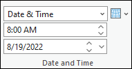
Learn more about date and time

Arrive Depart Date-Time Type

The Arrive Depart Date-Time Type drop-down list is available when the cost units are time based. From the drop-down list, choose whether a specific time and date value is given to indicate the time that the route or routes depart from their first stop. The primary reason for setting a specific time and date is to solve the analysis using dynamic traffic conditions or public transit schedules; however, to use traffic or public transit in the analysis, the network dataset or route service must include traffic data or public transit.

The options in the drop-down list are as follows:

• Not Using Time—Regardless of whether the network data source includes time-based data, the results are based on static travel times—the travel times on a network edge don't vary throughout the day. The Time of Day and Date text boxes are unavailable.

• Date & Time—Specify the time as a time of day and calendar date. The Time of Day and Date text boxes are available to provide this information.

• Day of Week—Specify a time of day and day of the week. The Time of Day and Date text boxes are available to provide this information.

• Today—Specify a time, and the day is assumed to be the current date. The Time of Day text box is available to provide the time of day, and the Date text box is set to Today and is unavailable so it can't be changed.

• Now—When you run the analysis, the time and date are set to the current time and date. This is useful if your network dataset is configured with live traffic data, and the routes are distributed to drivers for implementing immediately after running the analysis. The Time of Day and the Date text boxes are unavailable so they can't be changed.

Time of Day

Specify the depart time of the day.

See the Arrive Depart Date-Time Type section to see when this option is enabled.

Date

Specify the depart day of the week by typing one of the following values in the Date text box:

• Monday
• Tuesday
• Wednesday
• Thursday
• Friday
• Saturday
• Sunday

See the Arrive Depart Date-Time Type section to see when this option is enabled.

Reference Time Zone

From the Reference Time Zone drop-down list , you can choose which time zone to use in the analysis. The options are as follows:

• Local Time at Locations
• UTC (Universal Coordinated Time)

Note:

When solving a location-allocation analysis that spans across multiple time zones, the following requirements must be met:

• All facilities must be in the same time zone when specifying a start time and travel is from facility to demand.
• All demand points must be in the same time zone when specifying a start time and travel is from demand to facility.

Output Geometry

Use the options from the drop-down menu to choose how the output will display in the map.

Output Geometry Linear Shape Type

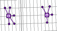
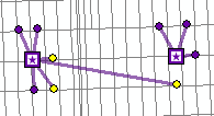
This control allows you to choose how the output will display in the map. The location-allocation analysis will always solve least-cost paths along the network, but these network paths cannot be displayed in the map. You can choose to represent the output as a straight line if you want to visualize the results in the map, or you can choose to not display any lines if you are only interested in the output fields in the Facilities, Demand Points, and Lines class tables.

• No Lines—No output linear shapes are generated.
• Straight Lines—Output simplified geometry as straight lines.

Drawing

Use the Symbology button to access the symbology pane for the active network analysis layer. You can configure the symbology for the sublayers of the active network analysis layer by choosing one of the following options:

• Single Color—This option is available for all network analysis layer types. All feature sublayers in the active network analysis layer except barriers will use the same single symbol with the specified color. For example, choosing a single color of blue for a Route layer will convert all the Stops and the Routes features to the same color of blue.
• Color Linked—This option is available for Route and Vehicle Routing problem layers. It applies a color scheme to the sublayers such that related features are symbolized with the same color. This symbology configuration symbolizes related features with the same color, making it easier to visually distinguish different routes and their associated features in the map. For example, for a Route layer with multiple routes, each route and the stops assigned to that route will be assigned matching colors.

Learn more about network analysis layer symbology

Filtering

You can filter the network analysis sublayers to only show features related to the selected features in the primary layer.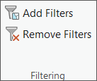

• Add Filters —Applies filters to sublayers of the network analysis layer to only show features related to the selected feature of the primary sublayer. Definition queries are automatically created and applied on the relevant sublayers. Every time the Add Filters button is clicked, a new definition query is created with the same name replacing the previous definition query.

  When a feature is selected in the primary sublayer Facilities, a definition query called Facilities is created on the Facilities sublayer (primary layer) and the related sublayers Lines and Demand Points.

• Remove Filters —Deletes the definition query on the primary and the related sublayers.