Common flood simulation workflows

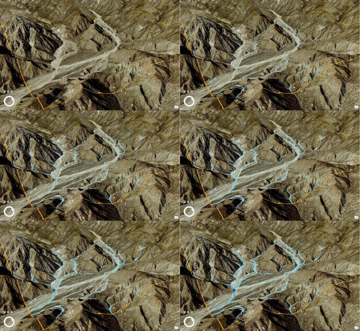
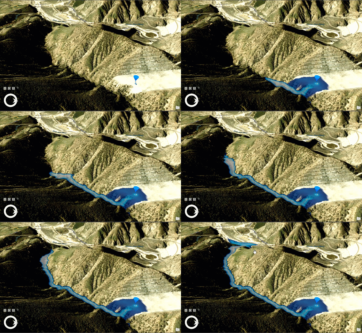
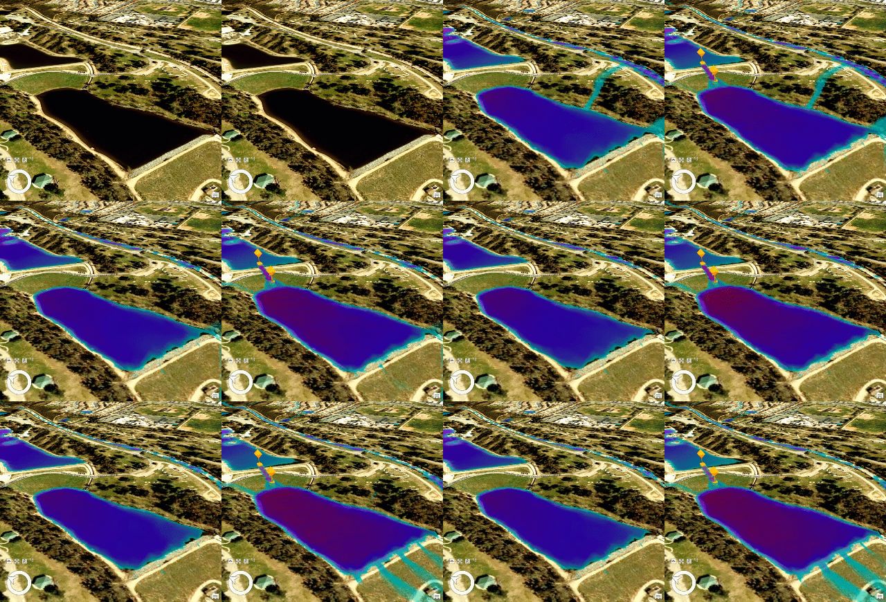
A flood simulation layer defines a scenario that will run for an area of interest inside a scene. The layer specifies incoming water volumes from rainfall, water source points and initial water depths, and can incorporate other elements that redirect the water such as channels, barriers, and infiltration properties. Each simulation runs against the terrain and features in the scene so you can use layer visibility, definition queries, and before-and-after elevation surfaces to investigate many scenarios. This topic outlines sample workflows that show how flood simulation can be used.

All flood simulation scenarios require you to author a scene containing the 3D world upon which the water will move. This includes a ground elevation surface and any important 3D vector elements that will impact water flow, such as buildings and dam walls. It is highly recommended that the elevation surface is carefully reviewed to remove anomalies and errors that impact water flow, such as bridges, cars, or trees that might have been captured into a DEM created from lidar. When the flood simulation is run, it will use the content of the scene directly as it is displayed.

Note:

The analytical results displayed by the simulation can be exported as temporal rasters for further use in GIS workflows, such as making maps, identifying areas of concern, and generating reports.

Model a storm using rainfall rates that vary over time

A simple scenario is to model how water from rainfall will flow and accumulate within an area of interest. This scenario can be run anywhere in the scene, in either local or global view mode. Begin with a scene containing relevant layers, such as a ground surface and buildings, and navigate the camera to the location you want to analyze.

1. Ensure a 3D scene is active.
2. In the Workflows group of the Analysis tab, expand the Simulation drop-down gallery of templates and select the Rainfall preset .

   The simulation toolbar to define the area of interest appears at the bottom of the 3D scene and the Centered Location creation tool is active by default, but any of the creation tools can be used.

3. Click the center of your intended study area, move the mouse outward, press the R key to open the Radius control, set the value to 2000 m, and press Enter.
4. On the simulation toolbar, click the Creation Simulation In Area button .

   A new simulation layer is added to the scene in the Simulations category of the Contents pane.

5. Click the Simulation tab to review the current properties of the simulation layer.

   Note:

   • Cell Size is 1 meter.
   • Duration is 1 hour.
   • Rainfall/hr rate is 40mm.

6. On the Simulation tab, in the Configuration group, set the Duration value to 00:30:00 (30 minutes).
7. In the Build group, click the Run button .

   Elevation values are extracted from the visible content in the scene, the Current time value starts progressing, and water begins to move and accumulate within the area of interest. Navigate the camera in and around the scene to get a closer look at the water movement.

8. Click the Pause button in the Playback group.

   The Current time value stops progressing and the water movement halts.

9. In the Contents pane, right-click the simulation layer and click the Configuration button to open the Configure Simulation pane.
10. In the Rainfall Rate table, click Split.
11. In the first row, set the Rate value to 5 and the Units/hr to inches (in).
12. In the second row, set the Rate value to 0.5 inches.
13. Click Split again.
14. Set the Rate for this new, third row to 0.1 inches.
15. Click Apply.
16. In the Build group of the Simulation tab, click the Run button .

    The simulation runs with extreme rainfall for 15 minutes, followed by reducing rates of water flow over the remaining 15 minutes as the hypothetical storm passes by.

17. After the simulation has fully played, click the Step Backward and Step Forward buttons in the Playback group of the Simulation ribbon to move through and explore the cached moments for the simulation.
18. Optionally, export the analysis to raster data by clicking the Analysis Results button in the Export group of the Simulation tab.
19. In the Export Simulation pane, set the Location to a folder on your local machine.
20. Click Export.

You now have a visual representation of where water flows and accumulates during a short but violent storm event. You can continue to experiment with different rainfall rates and other areas of interest. The exported raster data can be used with standard geoprocessing tools, such as the Raster Analysis toolbox and Overlay geoprocessing functions, to better understand the severity and extent of the impact.

Model the controlled venting of a dam

In this scenario, you will use a water source point to create a specific location where water flow is added into the simulation. This is useful for many use cases, such as venting a dam at a particular rate, representing a broken water pipe, or modeling the arrival of water from regions upstream from the area of interest.

1. Ensure a 3D scene is active.
2. In the Workflows group of the Analysis tab, expand the Simulation drop-down gallery of templates and select the Water Source preset.

   The simulation toolbar to define the area of interest appears at the bottom of the 3D scene and the Centered Location creation tool is active by default, but any of the creation tools can be used.

3. Click the center of your intended study area, move the mouse outward, and click again to set the general extent.

   Tip:

   The front of a dam wall, or a position on its spillway, is a good candidate for this location, though the analysis can be run anywhere.

4. On the simulation toolbar, click the Creation Simulation In Area button .

   A new simulation layer is added to the scene in the Simulations category of the Contents pane. It contains a single water source point at its center.

5. Click the Simulation tab to review the current properties of the simulation layer.

   Note:

   • Cell Size is a factor of the extent.
   • Duration is 1 hour.
   • Rainfall/hr rate is 40mm.

6. On the Simulation tab, in the Configuration group, set the Duration value to 00:12:00 (12 minutes).
7. In the Region group, click Modify .

   The selection handles appear. If they are not visible, click the Zoom to Simulation button to bring the entire area of interest into view.

8. Use the on-screen edit handles to move the area of interest so that the water source point is near the edge of, but still inside, the simulation area in order to include more of the expected downstream water flow.
9. On the simulation toolbar, click the Creation Simulation In Area button .

   The view updates to reflect this new area of interest boundary.

10. In the Contents pane, expand the subelement list to see the nodes in the Water Sources group.
11. Right-click Water Source 1 and click Modify .

    The modify overlay appears, titled Water Source 1.

12. In the overlay, change the Rate value to 200 and click the green check mark to apply your change.
13. In the Build group of the Simulation tab, click the Run button .

    Water starts emerging from the point location at 200 cubic meters per second.

    Note:

    Water sources are handled as a single cell. For a 1-meter cell size simulation, a flow rate of 200 cubic meters per second is applied as a tall column of water onto a single square meter of space. For less dramatic addition of water, add multiple nearby water source points and configure each to contain some fraction of the total required flow rate.

14. After the simulation has fully played, use the Step Backward and Step Forward buttons in the Playback group to move through and explore the cached moments for the simulation.
15. Optionally, export the analysis to raster data by clicking the Analysis Results button in the Export group.
16. In the Export Simulation pane, set the Location setting to a folder on your local machine.
17. Click Export.

You now have a visual representation of where water will flow from the water source point location. You can continue to experiment with different flow rates and other locations, including adding multiple water source points. The exported raster data can be used with standard geoprocessing tools, such as the Raster Analysis toolbox and Overlay geoprocessing functions, to better understand and explain where water will move from its starting location.

Review potential futures from a partially flooded state

In this scenario, you will use an initial-state water depth raster to load water on to the surface and then simulate potential futures from that state. This can be useful for what-if scenarios, such as modelling a potential levee burst or comparing the results from the worst-case and best-case rainfall predictions. This scenario requires a water depth raster, which could be modeled in a variety of ways. One option is to calculate the elevation surface difference between the terrain and a fixed elevation, such as filling up a dam, or using the output from another simulation run, such as the output from a rainfall simulation scenario or the predicted water levels from another flood simulation engine.

The following example shows exported results of the heavy storm scenario run above and will use its final state as the starting point for two new simulations. The original simulation layer is still in the active scene and the exported final-state analysis raster has also been added into the scene.

Two potential futures: On the left, the best-case result of only a light rain, and on the right, the worst-case result of heavy rain with a channel symbolizing dam overflow.

Create a best case scenario

Start by running the best-case scenario.

1. In the Contents pane, right-click the existing simulation layer and click Copy .
2. Right-click the Simulations category node and click Paste .
3. Click twice on the new simulation layer and rename it to Best Case.
4. Right-click the Best Case layer and click Configuration .
5. In the Configure Simulation pane, right-click the row header in the Rainfall Rate table and click Remove All Rows.
6. Click Append to add a new row.
7. In the new row, set the following values:
   • Duration—00:15:00
   • Rate—2
   • Units/hr—mm

   In this best-case scenario, the rainfall rate will remain steady at a slow 2 millimeters per hour.

8. Under the Starting Water Level heading, choose the final-state analysis raster layer from the drop-down gallery.

   All rasters in the Contents pane are listed.

9. Click Apply.
10. On the Simulation tab, in the Build group, click the Run button .

    Water is added to the surface of the ending state of the original simulation at a rate of 2 millimeters per hour.

Create a worst case scenario

Now that the best-case scenario has been run, the process must be repeated for the worst-case scenario.

1. In the Contents pane, right-click the Best Case simulation layer and click Copy .
2. Right-click the Simulations category node and click Paste .
3. Click twice on the new simulation layer and rename it to Worst Case.
4. Right-click the Worst Case layer and click Configuration .
5. In the Configure Simulation pane, in the Rainfall Rate table, update the Rate value to 25.

   In this worst-case scenario, the rainfall rate will remain high at 25 millimeters per hour.

   Other factors might also be at play for a worst-case scenario, such as the partial or full release of water from a levee or dam. Breaches in areas that contain water can be modeled as channel elements. Another possibility is the collapse of a bridge or the blocking of a stream, which can be modelled as barrier elements. Adding one or more of these elements into a simulation layer can provide even more variations for exploring potential futures.

6. Click Apply.
7. On the Simulation tab, in the Build group, click the Run button .

   As with the previous simulation, water is added to the surface of the ending state of the original simulation, but this time water is added at a rate of 25 millimeter per hour.

You now have comparative visual representations of how water will move from a given starting state using best- and worst-case parameters. You can continue to experiment with more alternate futures, such as the modelling of sandbags as barriers or the inclusion of upstream flow as water source points. For all options that are exported to rasters, the exported data can be used with standard geoprocessing tools, such as the Raster Analysis toolbox and Overlay geoprocessing functions, to compare and contrast a set of possible futures.