The Causal Inference Analysis tool estimates the causal effect between a continuous exposure variable and a continuous outcome variable by balancing confounding variables. The tool uses propensity score matching or inverse propensity score weighting to assign weights to each observation so that the confounding variables become uncorrelated with the exposure variable, isolating the causal effect between the exposure and outcome. The result is an exposure-response function (ERF) that estimates how the outcome variable responds to changes in the exposure variable. For example, you can estimate the average increase in corn yield (outcome) for different amounts of fertilizer (exposure) and factor out confounding variables such as soil type, farming techniques, and environmental variables that affect corn production. The ERF is displayed as a graphics layer and in the geoprocessing messages. Additionally, you can estimate the causal effect for individual observations and create goal-based objectives. For example, you can estimate the amount of fertilizer that each farm requires to produce a given amount of corn per year.
Causal inference analysis background
Causal inference analysis is a field of statistics that models cause-and-effect relationships between two variables of interest. One variable (called the exposure or treatment variable) directly changes or affects another variable (known as the outcome variable). Correlations are often used as a measure of how changes to one variable are associated with changes to the other variable; however, correlation doesn't necessarily mean that one variable causes the other. It could be that they're both influenced by other factors. For example, the relationship between ice cream sales and sunscreen sales might have a strong positive relationship. However, you cannot conclude that higher ice cream sales are causing higher sunscreen sales. Other factors such as temperature, UV index, or month of the year must be accounted for before drawing causal conclusions. The factors that affect both the exposure and outcome variables are called confounding variables, and it is essential that they be included and accounted for to accurately capture the cause-and-effect relationship between the exposure and outcome variables.
A causal analysis starts with a hypothesis grounded in research or common knowledge. For example, consider the effect of exercise on health. There is evidence and common knowledge that regular exercise can improve health, but the variables also depend on numerous other confounding variables such as food habits, lifestyle choices, and access to safe exercise areas. In situations like this, causal inference analysis can be used to isolate the effect of the exposure variable (for example, daily time spent on exercise) on the outcome variable (for example, heath outcome) after accounting for various important confounding variables.
In designed experiments, confounding variables are controlled using randomized controlled trials (RCTs). RCTs are widely used in clinical research, and they involve participants being randomly assigned different levels of exposure, and their outcomes are compared. For example, one individual exercises for 10 minutes every day, another exercises for one hour, and another doesn't exercise at all. Because their exposure variables were assigned randomly, any differences in the health outcome within the group cannot be attributed to anything other than the exposure variable.
However, in real world scenarios, it is often impossible or unethical to create controlled experimental groups. For example, to study the effect of pollution on depression, you cannot ethically expose people to high pollution to see what happens to their depression. Instead, you can only observe the pollution level that people already experience and observe their depression rates. Causal inference analysis can then be used to model the causal relationship from the observational data by mimicking a controlled experimental design. It does this by estimating a propensity score for each observation, and the propensity scores are used to estimate a set of balancing weights for the observations. The balancing weights are configured in such a way that they maintain the causal relationship between the exposure and outcome variables, but they remove the effect of the confounding variables on the exposure variable, allowing unbiased estimation of the causal relationship. The resulting weighted observations have analogous properties to a dataset collected through an RCT, and you can make inferences from it in many of the same ways you can for datasets collected through a designed experiment.
Two common ways to estimate balancing weights are propensity score matching and inverse propensity score weighting. In propensity score matching, each observation is matched with various other observations that have similar confounding variables (measured by similarity of their propensity scores) but have different exposure values. By comparing the outcome value of an observation to the outcome values of its matches, you can see what the observation's outcome value might have been if it had different exposures. The balancing weight assigned to each observation is the number of times that it was matched to any other observation. In inverse propensity score weighting, balancing weights are assigned by inverting the propensity scores and multiplying by the overall probability of the exposure. This procedure increases the representation of uncommon observations (observations with low propensity score) and decreases the representation of common observations (high propensity scores) so that the influence of the confounding variables is kept in proportion across all values of the exposure variable.
The balancing weights from propensity score matching or inverse propensity score weighting do not always sufficiently balance the confounding variables, so their weighted correlations are calculated compared to a threshold value. If the correlations are under the threshold (meaning the correlation is low), they are determined to be balanced, and an ERF is estimated. However, if the balancing weights do not sufficiently balance the confounding variables, the tool will return an error and not produce an ERF.
Example applications
The following are example applications of the tool:
- Investigate how exposure to tobacco product advertisements affects tobacco use in teens in the United States. In this example, the exposure variable is the amount of exposure to advertising for each teen, and the outcome variable is the amount of tobacco consumed by each teen over a given time period. The confounding variables should be any other variables that are known or suspected to be related to the exposure to or use of tobacco products in teens, such as socioeconomic variables, direct exposure to tobacco products from family or friends, price of tobacco products, and availability of tobacco products. Many exposure variables could be chosen to investigate teen tobacco use (such as direct exposure to tobacco products from family members), but tobacco product advertising is a useful exposure variable because if it is found to cause a large increase on teen tobacco use, the amount of advertising can be reduced through regulation. Reducing tobacco product use among adult family members, however, would be more difficult.
- Estimate the causal effect of the amount of fertilizer on corn yield in precision agriculture while controlling for the type of soil, farming techniques, environmental variables, and other confounding variables of each farming plot. For example, how much extra corn would be produced if each farm increased the amount of fertilizer by 10 percent?
- Estimate the causal effect between blood pressure and risk of heart attack, controlling for confounding variables such as age, weight, sociodemographic variables, and health-care access.
- In spatial data, distances to other features are often useful exposure variables. For example, the distance to grocery stores, green areas, and hospitals cause changes in other variables: being farther from a grocery store reduces food access, being farther from a hospital reduces health-care access, and so on. For similar reasons, spatial variables and distances to other features are also frequently important confounding variables even when the exposure and outcome variables are not spatial variables.
However, causal inference analysis has a number of limitations and assumptions that must be fulfilled for the estimates of the causal effects to be unbiased and valid. The following are some of the assumptions and limitations of causal inference analysis:
- All important confounding variables must be included. This is a strong assumption of causal inference analysis, and it means that if any variables that are related to both the exposure and outcome variables are not included as confounding variables, the estimate of the causal effect will be biased (a mixture of the causal effect and the confounding effect of any missing confounding variables). The tool cannot determine whether all important confounding variables have been included, so it is critical that you consider which confounding variables you include. If there are important confounding variables that are not available, interpret the results with extreme caution or do not use the tool.
- The correlations between the confounding variables and the exposure variable must be removed in order to isolate the causal effect. In causal inference analysis, removing the correlations between the confounding and exposure variables is called balancing, and the tool uses various balancing procedures. However, it cannot always sufficiently remove the correlations between the confounding and exposure variables. If the balancing procedure does not sufficiently balance the confounding variables, the tool will return an error and not estimate an ERF. See Tips to achieve balanced confounding variables for more information about the error and how to resolve it.
- The ERF cannot extrapolate outside of the range of exposure values that were used to estimate it. For example, if the exposure variable is mean annual temperature, you cannot estimate new outcomes for temperatures larger than the ones in the sample. This means, for example, that you may not be able to predict outcomes in the future when mean temperatures will exceed any current mean temperatures. Additionally, the tool trims (removes from analysis) the top and bottom 1 percent of exposure values by default, so the range of the ERF will be more narrow than even the exposure values of the observations in the sample.
Tool outputs
The tool creates a variety of outputs you can use to investigate the causal relationship between the exposure and outcome variables. The results are returned as a graphics layer, geoprocessing messages, output features (or table), and an output ERF table.
Exposure-response function
The primary result of the tool is the ERF that estimates how the outcome variable responds to changes in the exposure variable. The ERF estimates the new population average (the average of all members of the population) of the outcome variable if all members of the population changed to have the same exposure variable value but kept all their existing confounding variables. For example, for all U.S. counties, if the exposure variable is PM2.5 and the outcome variable is asthma hospitalization rates, the ERF estimates how the average national asthma hospitalization rate would change if the national PM2.5 level was increased or decreased while keeping all other variables (such as sociodemographic variables) the same as they were before the change in PM2.5.
When run in an active map, a graphics layer will be added to the map displaying the ERF. The same ERF image is also displayed in the messages.
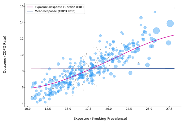
The pink curve is the ERF between the exposure (x-axis) and outcome (y-axis) variables. The observations are shown as light blue bubbles in the background of the scatterplot, and larger bubbles indicate that the feature had a larger balancing weight and contributed more to the estimation of the ERF. For propensity score matching, if the observation has no matches, it is drawn as a light gray point. Trimmed observations are not shown in the chart.
The ERF also contains a blue horizontal line showing the average value of the outcome variable so that it can be compared to the estimated average for various levels of the exposure variable. For example, in the image above, if all counties changed their smoking prevalence to the same value below approximately 17.5 (where the mean line crosses the ERF), the overall COPD rate would decrease from the current level. Similarly, the overall COPD rate would increase if all countries changed to a smoking prevalence higher than 17.5.
You can also use the Output Exposure-Response Function Table parameter to create a table of the ERF. If created, the table will contain 200 evenly spaced exposure values between the minimum and maximum exposure along with the corresponding response (outcome) value. If any target exposure or target outcome values are provided, they will also be appended to the end of the table along with the estimated exposure or response value.
Confounding variable balance statistics
The Balance Results section of the messages displays the original and weighted absolute correlations between each confounding variable and the exposure variable. This allows you to see whether the balancing weights effectively reduced the original correlation between the confounding variables and the exposure variable. If the weights are effective at balancing, the weighted correlations should be lower than the original correlations. The final row in the message table shows the mean, median, or maximum absolute correlation, depending on the value of the Balance Type parameter.
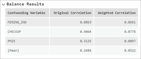
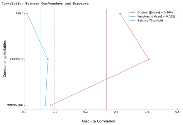
The Correlation Between Confounders and Exposure message chart displays the same information as the table, except in a vertical line chart. For each confounding variable, the original correlations are connected by a red line, and the weighted correlations are connected by a blue line. The original and weighted aggregated correlations are also drawn as vertical red and blue bars, respectively. If the weights effectively balance the confounding variables, the blue lines should generally be to the left of the red lines. The balance threshold is drawn as a vertical dashed line, allowing you to see how close the correlations were to the threshold. For example, in the image below, two of the confounding variables started with relatively large correlations (above 0.3 and 0.4, respectively), but the balancing weights reduced the correlations to less than 0.1. The third confounding variable started with a low correlation (slightly less than 0.1), but the balancing weights still reduced the correlation by a small amount. Overall, the mean correlation reduced from nearly 0.27 to under 0.05.
See the Check for balanced confounding variables section below for more information about confounding variable balance.
Parameter tuning results
The messages also contain sections summarizing various tuning parameters that are used to estimate the ERF. Depending on the parameters specified in the tool, the following sections may be displayed:
- Trimming Results—The original number of observations (after removing any records with null values), the number of observations that were removed by exposure trimming, the number of observations removed by propensity score trimming, and the final number of observations remaining after trimming are displayed.
- Matching Grid Search Results—For propensity score matching, the results of the matching parameter search are displayed. The tool will use various combinations of number of exposure bins and relative weight of propensity score to exposure (scale) and display the resulting weighted correlations for each combination. The combination that results in the lowest weighted correlation (best balance) is highlighted in bold.
- Transformation Balancing Results—For the regression propensity score model, the confounding variable transformations that were used to attempt to find balance, along with the weighted correlation for each transformation combination, are displayed. The transformation combination that results in the lowest weighted correlation is highlighted in bold.
- Gradient Boosting Balancing Results—For the gradient boosting propensity score model, the results of the gradient boosting grid search are displayed. The tool tries nine combinations of number of trees and learning rate and displays the weighted correlations for each combination. The combination that results in the lowest weighted correlation is highlighted in bold.
- Parameters Resulting in Best Balance—For propensity score matching, the number of exposure bins and relative weight of propensity score to exposure (scale) that resulted in the best confounding variable balance are displayed. For gradient boosting, the number of trees, learning rate, and random number generator seed value that resulted in the best balance are displayed.
- Balance Results—The original and weighted correlations for each confounding variable, along with the mean, median, or maximum correlations are displayed. If transformations were used, the transformation is also shown for each confounding variable.
See the Estimate optimal balancing parameters section below for more information about how many of the values in the messages are determined.
Output features
The output features or table contains copies of the exposure, outcome, and confounding variables, along with the propensity scores, balancing weights (match counts or inverse propensity score weights), and a field indicating whether the record was trimmed. When added to a map, the output features will draw based on the balancing weight. This allows you to see if there are any spatial patterns to the weights, which may indicate that certain regions are being over- or under-represented in the results.
If you provide any target exposure or outcome values, each provided value will create two additional fields on the output. For target exposure values, the first field contains the estimated outcome value if the observation received the target exposure, and the second field contains the estimated change in the outcome variable. Positive values indicate that the outcome variable will increase, and negative values indicate that the outcome variable will decrease. For target outcome values, the first field contains the exposure value that would result in the target outcome, and the second field contains the required change in the exposure variable to produce the target outcome.
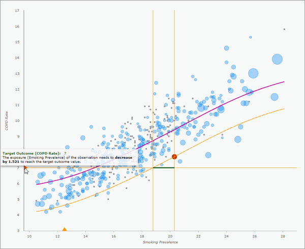
If you create local ERF pop-up charts, each output record will display the local ERF in the pop-up pane. Any target outcome or exposure values are shown as orange triangles on the x- and y-axes. You can click the triangles to turn on and off horizontal or vertical bars to see where the value crosses the local ERF. Additionally, you can hover over the triangles to see information about the required changes in exposure or outcome to reach the target. See Estimate local causal effects for more information.
If you create bootstrapped confidence intervals for the ERF, two additional fields will be created containing the number of times the observation was selected in a bootstrap sample and the number of times that the observation was included in a bootstrap sample that attained balance. It is recommended that you look for spatial patterns in both fields. If some regions contain many more balanced bootstrap samples than other regions, the confidence intervals may be biased (usually resulting in confidence intervals that are unrealistically narrow). See Bootstrapped confidence intervals for more information.
Propensity scores
A fundamental component of causal inference analysis is the propensity score. A propensity score is defined as the likelihood (or probability) that an observation would take its observed exposure value, given the values of its confounding variables. A large propensity score means that the exposure value of the observation is common for individuals with similar confounding variables, and a low propensity score means that the exposure value is uncommon for individuals with similar confounding variables. For example, if an individual has high blood pressure (exposure variable) but has no risk factors (confounding variables) for high blood pressure, this individual would likely have a low propensity score because it is relatively uncommon to have high blood pressure without any risk factors. Conversely, high blood pressure for an individual with many risk factors would have a larger propensity score because it is a more common situation.
Two approaches to causal inference analysis use the propensity score: propensity score matching and inverse propensity score weighting. Each approach assigns a set of balancing weights to each observation that are then used to balance the confounding variables (see the Check for balanced confounding variables section below for more information).
Propensity score matching
Propensity score matching attempts to balance the confounding variables by matching each observation with various observations that have similar confounding variables but different exposures. By comparing the outcome value of the observation to the outcomes of the matching observations, you see the outcomes the observation might have had if it had a different exposure (but kept the same confounding variables). After finding matches for all observations, the balancing weight assigned to each observation is the number of times that the observation was matched to any other observation. For example, if an observation is not the match of any other observation, the balancing weight will be zero, and if the observation is the match of every other observation, the balancing weight will be equal to the number of observations.
Propensity score matching for continuous exposure variables is relatively complicated and is fully described and derived in the fourth and fifth items in the References section below. The following is a brief summary of the matching procedure:
The procedure begins by dividing the observations into equally spaced bins based on the exposure variable (similar to the bins of a histogram) using the value of the Number of Exposure Bins parameter. Propensity score matching is performed within each bin by comparing the propensity scores of the observations in the bin to the counterfactual propensity scores of every other observation. Counterfactual propensity scores are the propensity scores that an observation would have had if it had the same confounding variables but instead had different exposures (in this case, the center values of each exposure bin). Matches within each bin are determined by finding the observation in the exposure bin whose propensity score is closest to the counterfactual propensity scores of each of the other observations. However, because the exposure values of the observations in the bin will not generally align with the bin center, an additional penalty is added based on the difference between the exposure value and the center of the exposure bin. The amount that is penalized is determined by the value of the Relative Weight of Propensity Score to Exposure parameter (called the scale parameter in the references), and the overall match is the observation with the lowest weighted sum of the absolute differences in propensity scores (propensity score minus counterfactual propensity score) and exposure (raw exposure minus bin center value).
Inverse propensity score weighting
Inverse propensity score weighting assigns balancing weights to each observation by inverting the propensity score and multiplying by the overall probability of having the given exposure. This approach to causal inference provides higher balancing weights to observations with low propensity scores and lower balancing weights to observations with high propensity scores. The reasoning behind this weighting scheme is that the propensity score is a measure of how common or uncommon the exposure value is for the particular set of confounding variables. By increasing the influence (increasing the balancing weight) of uncommon observations (observations with low propensity scores) and decreasing the influence of common observations, the overall distributions of confounding variables are kept in proportion across all values of the exposure variable.
Note:
Kernel density estimation (KDE) is used to estimate the overall probability of the exposure value. The KDE uses a Gaussian kernel with Silverman's bandwidth, as implemented in the scipy.stats.gaussian_kde function of the SciPy Python package.
Propensity score estimation
The Propensity Score Calculation Method parameter allows you to specify how the propensity scores will be estimated. Each method builds a model that uses the confounding variables as explanatory variables and the exposure variable as the dependent variable. Two propensity score calculation methods are available:
- Regression—Ordinary least-squares (OLS) regression is used to estimate the propensity scores.
- Gradient boosting—Gradient boosted regression trees are used to estimate the propensity scores.
For the regression model, predictions are assigned probabilities by assuming normally distributed standardized residuals. The gradient boosting model does not naturally produce standardized residuals, so the tool builds a second gradient boosting model to predict the absolute value of the residuals of the first model, which provides an estimate of the standard error. KDE (the same as in inverse propensity score weight above) is then used on the standardized residuals to create a standardized residual distribution. This distribution can then be used to estimate propensity scores for all combinations of exposure and confounding variable values.
Both regression and gradient boosting rescale all variables to be between 0 and 1 before building their respective models.
Check for balanced confounding variables
For the ERF to be an unbiased estimate of the causal effect, all confounding variables must be included and balanced, meaning that confounding variables must be uncorrelated with the exposure variable. Because confounding variables are correlated with the exposure variable by definition, the original confounding variables will always be unbalanced. However, the purpose of the balancing weights (from propensity score match counts or inverse propensity score weights) is to weight each observation in such a way that the weighted observations become balanced, but the causal relationship between the exposure and outcome variables is maintained, allowing unbiased estimation of the ERF.
To determine whether the balancing weights effectively balance the confounding variables, weighted correlations are calculated between each confounding variable and the exposure variable. The absolute values of the weighted correlations are then aggregated and compared to a threshold value. If the aggregated correlation is less than the threshold, the confounding variables are determined to be balanced. You can specify the aggregation type (mean, median, or maximum absolute correlation) using the Balance Type parameter and provide the threshold value in the Balance Threshold parameter. By default, the tool will calculate the absolute mean correlation and use a threshold value equal to 0.1.
Note:
For continuous confounding variables, the weighted correlations are calculated using a weighted Spearman's rank correlation coefficient. This correlation is similar to a traditional Pearson correlation coefficient, but it uses the weighted ranks of the variables in place of raw values. Using ranks makes the correlation more robust to outliers and oddly shaped distributions. For categorical confounding variables, the weighted correlations are calculated using a weighted eta statistic that uses weighted ranks of the exposure variable. The eta statistic is a close equivalent of absolute Pearson correlation for categorical variables (both can be defined as the square root of R-squared, the coefficient of determination), and using weighted ranks in place of raw exposure values makes it a close equivalent to the absolute value of a weighted Spearman correlation.
Tips to achieve balanced confounding variables
If the balancing weights do not sufficiently balance the confounding variables, the tool will return an error and not produce an ERF; however, various messages are still displayed with information about the weighted correlations of each confounding variable. When you encounter this error, review the messages to determine how much the balancing weights reduced the correlations and how close the weighted correlation was to the balance threshold.
When the tool fails to achieve balance, consider whether you are missing any relevant confounding variables, and include any that you are missing. Next, try different options for the Propensity Score Calculation Method and Balancing Method parameters. However, for some datasets, there may be no combination that achieves balance.
In general, the larger the original correlations of the confounding variables, the more difficult it is to balance them. For strongly correlated confounding variables, large sample sizes may be necessary to achieve sufficient balance. For categorical confounding variables, the more categories, the more difficult it is to balance. It may be necessary to combine some of the categories, especially if there is little variation of the exposure variable or a small number of observations (generally fewer than five) in each category.
However, if you can tolerate the introduction of bias into the ERF, you can achieve balance by increasing the balance threshold or using a more lenient balance type.
In general, a lower balance threshold value indicates less tolerance for bias in the estimation of the causal effect; however, it is more difficult to achieve balance with lower thresholds. For the balance type, using the mean of the correlations ensures that the confounding variables are balanced on average, but it still allows some confounding variables to have large correlations if there are enough of them with lower correlations to bring the average below the threshold. The maximum option is the most conservative and requires that every confounding variable be under the threshold; however, if even a single confounding variable is slightly above the threshold, the confounding variables will be deemed unbalanced. The median option is the most lenient, and it allows up to half of the correlations to be very large and still be considered balanced.
Estimate optimal balancing parameters
Achieving confounding variable balance can often be difficult, so the tool will attempt various optimizations and searches to find tuning parameters that result in confounding variables that are as balanced as possible. The optimizations that are performed depend on various parameters of the tool, and they are described in the following sections.
Matching parameter search
In propensity score matching, the matching results depend on the values of the Number of Exposure Bins and Relative Weight of Propensity Score to Exposure parameters, but it is difficult to predict the values that will result in the best balance. Further, small changes in one of the values can result in large changes of the other, so it is especially difficult to find a pair of values that works effectively. If values are not provided for the parameters, the tool will try various combinations and display the results as a table in the messages. In the table, the rows are the number of exposure bins, and the columns are the relative weights (often called the scale). The weighted correlation of each combination is shown in the grid, and any combination that achieved balance will have an asterisk next to the value. The combination that results in the lowest weighted correlation (best balance) is highlighted in bold. As shown in the image below, the weighted correlations can vary substantially for different values of the two parameters.
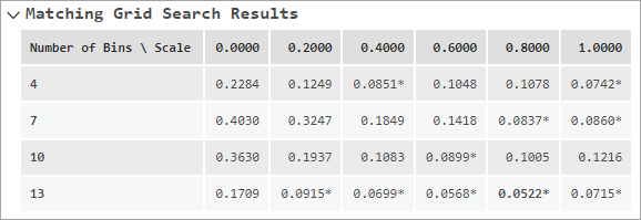
The tool attempts relative weights ranging from 0 to 1 by 0.2, but the numbers of exposure bins that are tested depend on the number of observations. The tested values range between the fourth root and two times the cubic root of the number of observations. The tested values will increment evenly by no less than three, and no more than 10 values will be tested.
Regression transformations
When using regression to calculate propensity scores, if the confounding variables do not balance, various transformations will be applied to any continuous confounding variables. If at any point the confounding variables achieve balance, the process ends and the current set of transformations will be used to build the ERF.
The process begins with the confounding variable that is least balanced (largest weighted correlation) and applies a sequence of transformations. The transformation that achieves best balance is kept, and the process repeats on the next confounding variable. This continues until all confounding variables have been tested with all transformations, and if the confounding variables are still not balanced, the tool will return an error and not produce an ERF.
The following transformations will be performed, with some restrictions on the values of the confounding variables being transformed:
- Natural logarithm—Only for confounding variables with positive values
- Square—Only for confounding variables with nonnegative values
- Square root—Only for confounding variables with nonnegative values
- Cube
- Cubic root
The transformations that resulted in best balance will be shown in the Balance Results section of the messages, and the full history of transformation attempts will be displayed in the Transformation Balancing Results section.
In propensity score matching, the number of exposure bins and relative weight values from the original (untransformed) confounding variables will be used for all transformation combinations. This is to prevent very long calculation times by repeating the matching parameter search for every transformation combination. The square transformation is restricted to nonnegative values so that the ordering of the confounding variable values does not change before and after the transformation, which is important when reusing the number of exposure bins and relative weight determined from the original observations.
Gradient boosting parameter search
When using gradient boosting to calculate propensity scores, various combinations of the number of trees and learning rate are tested. If at any point the confounding variables achieve balance, the process ends and the current number of trees and learning rate are used. The process tries up to nine combinations: number of trees equal to 10, 20, and 30 trees and learning rates equal to 0.1, 0.2, and 0.3.
The number of trees and learning rate resulting in the best balance will be displayed in the Parameter Resulting in Best Balance section of the messages, and the full history of parameter combinations will be shown in the Gradient Boosting Balancing Results section.
Unlike the regression transformations, the matching parameter search for the number of exposure bins and relative weight will be repeated for each combination of number of trees and learning rate. A deeper search is performed because small changes in any of these four parameters can cause large changes in the optimal values of the others.
Estimate the exposure-response function
The balancing procedure assigns balancing weights (match counts or inverse propensity score weights) to each observation, and these weights are the foundation for estimating the exposure-response function. The weighted observations (sometimes called a pseudopopulation) each have an exposure value, outcome value, and weight, and the goal is to fit a smooth curve (the ERF) to the weighted observations. When estimating the ERF, each observation influences the estimation proportionally to its weight. In other words, an observation with a weight equal to three contributes as much as three observations that each have weight equal to one. Similarly, any observation with weight equal to zero will have no impact on the ERF, effectively filtering out the observation.
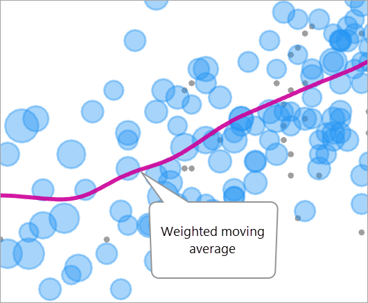
For a given value of the exposure variable (x-axis), the associated response value (y-axis) is estimated as a weighted moving average (sometimes called a kernel smoother) of the outcome values of the observations. The weights in the weighted average are the balancing weights multiplied by the weight from a Gaussian kernel trimmed at three standard deviations.
When this procedure is performed on all values of the exposure variable, the result is a smooth curve that passes through the observations and is pulled toward the observations with the largest weights.
Bandwidth estimation
The kernel in the ERF formula depends on a bandwidth value (the standard deviation of the Gaussian kernel) that controls the smoothness of the ERF curve, and specifying an appropriate bandwidth is critical to produce a realistic and accurate ERF. Larger bandwidth values result in smoother ERFs for the same set of weighted observations. The following image shows three bandwidth values used for the same observations:
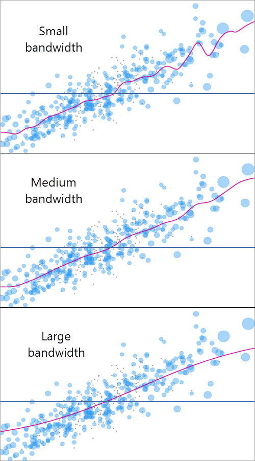
You can use the Bandwidth Estimation Method parameter to choose how to estimate a bandwidth value. Three bandwidth estimation methods are available:
- Plug-in—A fast rule-of-thumb formula is used to estimate a bandwidth value. This option is the default, calculates quickly, and generally produces accurate and realistic ERFs. The method is a weighted variant of the methodology from Fan (1996) and derives the bandwidth value from the second derivative of a weighted fourth-order global polynomial fitted to all observations.
- Cross validation—The bandwidth value that minimizes the mean square cross validation error is used. This option takes the longest to calculate but is the most well-founded in statistical theory. However, for large datasets, cross validation has a tendency to estimate bandwidth values that are too small and produce ERFs that are too curvy.
- Manual—The custom bandwidth value provided in the Bandwidth parameter is used. This option is recommended when the other options produce bandwidth values that result in ERFs that are too smooth or too curvy. In this case, review the bandwidth values estimated by the other methods and make any needed corrections to adjust the smoothness.
The estimated bandwidth value will be printed at the bottom of the messages.
Note:
For the plug-in and cross validation methods, if the estimated bandwidth value is less than the largest gap between exposure values, the largest gap will be estimated instead. This is to ensure that every exposure value has sufficient data for the weighted average. To use smaller bandwidth values, provide a manual bandwidth value.
Estimate local causal effects
You can create local ERFs for each record in the output feature or table by checking the Enable Exposure-Response Pop-ups parameter. If checked, the output will contain an ERF chart in the pop-ups of each output feature or table record. The pop-ups display how the outcome variable for the individual observation is estimated to respond to changes in its exposure variable. The local ERF takes the same shape as the global ERF, but it is shifted up or down to pass through the individual observation. Additionally, if any target outcome or exposure values are provided, they are shown in the pop-up charts along with the required changes in exposure or outcome in order to achieve the targets.
Creating local ERFs or using target exposure or outcome values requires making an additional assumption of a fixed exposure effect for all observations. This is a strong assumption, and violating it can lead to biased or misleading results. The fixed exposure effect assumption implies that the effect of the exposure on the outcome is constant across all individuals in the population. In other words, given their starting exposure, increasing the exposure by a fixed amount changes the outcome in the same way for everyone, regardless of the levels of any other variable (including, but not limited to, the measured confounders). For example, increasing the amount of fertilizer from 150 lb per acre to 175 lb per acre would need to increase corn yield by the same amount on all farms, regardless of their current corn yield, type of soil, farming techniques, or other confounding variables.
This assumption is reasonable when there are no effect modifiers, that is, variables that affect how the outcome responds to the exposure on an individual level. However, sociodemographic variables such as gender, race, or educational levels are often effect modifiers, and they are typically included as confounding variables in causal inference models. This works well to average out the effect modification across all levels of the modifying variable, allowing estimation of a global average causal effect (the ERF). However, the global ERF doesn't represent any specific subgroup defined by the levels of the effect modifier. For example, a job training program might show increased job offers with more training hours. However, job offers plateau after certain training hours in predominantly Black or Hispanic neighborhoods, potentially hinting at systemic hiring discrimination. Therefore, the global ERF may unintentionally mask disparities faced by these communities. The global ERF represents the effect of exposure on outcomes averaged across the whole population; however in the presence of effect-modifying variables, the global ERF may not accurately represent the effect of exposure on outcomes in predominantly Black or Hispanic areas.
Local ERFs are not valid when the model contains effect modifiers. One approach to dealing with the effect modifiers is stratification, which involves dividing up the observations into strata (or subgroups) based on the values of the modifying variable. By separating the effect modifiers by strata and building independent ERFs for each strata, you can examine the relationship between the exposure and the outcome within each group separately. This allows you to see if the effect of the exposure on the outcome differs across the different levels of the effect modifier.
Bootstrapped confidence intervals
You can create 95 percent confidence intervals for the ERF using the Create Bootstrapped Confidence Intervals parameter. If created, the confidence intervals will draw as dashed lines above and below the ERF in the output graphics layer and messages. If an output ERF table is created, it will also contain fields of the upper and lower confidence bounds.
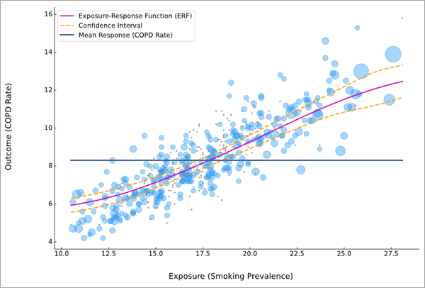
The confidence intervals are bounds on the population average of the outcome variable for any given value of the exposure variable. Because population averages have less variability than individual members of the population, most points of the scatterplot will generally not fall within the confidence intervals, but this is not indicative of a problem. For similar reasons, the confidence intervals are only applicable to the global ERF, and they cannot be applied to any local ERFs.
The confidence intervals are created using M-out-of-N bootstrapping. This procedure entails randomly sampling M observations from the N observations, where M=2*sqrt(N), as recommended by DasGupta (2008). The tool then performs the entire algorithm (optimal parameter search, propensity score estimation, balance test, and ERF estimation) on the random bootstrap sample. The resulting ERF will usually be similar to the original ERF, but it will not be exactly the same. By repeating this process many times, you can see how much the ERF varies when taking different random samples of the observations. The variation of the resulting ERFs is what drives the creation of the confidence intervals.
If a bootstrap sample does not achieve balance (as determined by the balance type and balance threshold), the bootstrap sample will be discarded. The tool will continue to perform bootstraps until 5*sqrt(N) bootstrap samples achieve balance. This value is derived so that every observation is expected to be included in at least 10 balanced bootstrap samples on average. This allows stable estimates of the upper and lower bounds across the entre range of exposure. If there are still not enough balanced bootstraps after 25*sqrt(N) bootstrap attempts, confidence intervals will not be created, and a warning message will be returned.
While the confidence intervals capture many sources of uncertainty of the ERF, it is important to note that to create confidence intervals that truly correspond to upper and lower bounds of the causal effect, all potential sources of uncertainty must be accounted for. The bootstrap procedure in this tool incorporates the uncertainty of the balancing procedure and ERF estimation, but it cannot account for other possible sources of uncertainty, such as imprecision in the values of the variables or the choice of the functional form of the ERF (a weighted moving average, as opposed to a spline or global polynomial, for example). Additionally, the confidence intervals will become arbitrarily narrow as you increase the number of observations, but do not take this to mean that the ERF is a perfect characterization of the causal effect.
When bootstrapped confidence intervals are created, the output features or table will contain two fields related to the bootstraps. The first field contains the number of times the observation was selected in a bootstrap sample, and the second field contains the number of times the observation was included in a bootstrap sample that achieved balance and an ERF was estimated. These fields will be created even if not enough bootstrap samples achieve balance to estimate the confidence intervals. For output features, the values of the first column should show few spatial patterns, except around the perimeter of the features. However, if there are spatial patterns in the second field, this may indicate a spatial process that is not being accounted for. For example, if most balanced bootstrap samples come from particular regions of the data, these regions are being over-represented in the confidence intervals, and the intervals may be unrealistically narrow. If you see spatial patterns in the counts of balanced bootstraps samples, consider including a spatial confounding variable (such as a geographical region) to account for the missing spatial effect.
For input tables, each bootstrap selects M observations randomly and uniformly. The sampling is with replacement, so the same observation can be selected multiple times in the same bootstrap. For feature input, the bootstrap samples are generated by selecting a single feature randomly and including it and its eight closest neighboring features in the sample. This random selection repeats with replacement until at least M observations are included in the bootstrap sample. The same features can be randomly selected multiple times and can be included as neighbors multiple times. Using random neighborhoods rather than completely random selection helps correct for unmeasured spatial confounding (though you are still encouraged to correct for spatial confounding by including spatial variables as confounding variables).
Because ERFs cannot expand beyond the range of exposure values used to build them, the ERF of each bootstrap sample will only be created between the minimum and maximum exposure of the observations in the random sample. This means the highest and lowest exposure values will frequently not be within the range of the randomly sampled values, so fewer bootstrapped ERFs are created for the most extreme exposure values.
After all bootstraps complete, the 95 percent confidence intervals are created by assuming a T-distribution of the bootstrapped ERF values for each exposure value. The variance of the ERF values is rescaled by multiplying by (M/N) to adjust for only sampling M values, and the degree of freedom is the number of bootstrapped ERFs that could be generated for the exposure value, minus one. Additionally, the widths of the confidence intervals are smoothed using the same kernel smoother as was used to estimate the original ERF (equal weights with plug-in bandwidth). The smoothed width is then added and subtracted from the original ERF to produce the upper and lower confidence bounds. If an output ERF table is created, it will contain fields with the smoothed standard deviation (smoothed width divided by critical value) and the number of bootstrapped ERFs that could be generated for the exposure value.
References
DasGupta, Anirban. 2008. "Asymptotic Theory of Statistics and Probability." New York, NY. Springer. ISBN 978-0-387-75971-5. https://doi.org/10.1007/978-0-387-75971-5.
Fan, Jianquin. 1996. "Local Polynomial Modeling and Its Applications: Monographs on Statistics and Applied Probability 66." (1st ed.). Routledge. https://doi.org/10.1201/9780203748725.
Imbens, Guido and Donald B. Rubin. 2015. "Causal Inference for Statistics, Social, and Biomedical Sciences: An Introduction." Cambridge: Cambridge University Press. https://doi.org/10.1017/CBO9781139025751.
Khoshnevis, Naeem, Xiao Wu, and Danielle Braun. 2023. "CausalGPS: Matching on Generalized Propensity Scores with Continuous Exposures." R package version 0.4.0. https://CRAN.R-project.org/package=CausalGPS.
Wu, Xiao, Fabrizia Mealli, Marianthi-Anna Kioumourtzoglou, Francesca Dominici, and Danielle Braun. 2022. "Matching on Generalized Propensity Scores with Continuous Exposures." Journal of the American Statistical Association. https://doi.org/10.1080/01621459.2022.2144737.